

I spent the better part of a Tuesday afternoon in a repair bay last month staring at a Freightliner that had zero active fault codes, a battery voltage that never dipped below twelve-point-six volts, and a CAN bus that would randomly drop frames for six to eleven seconds. No pattern. No correlation with temperature, engine load, or road vibration. The fleet manager had already thrown a reman ECU, two NOx sensors, and an instrument cluster at the problem. Total bill: four thousand two hundred dollars in parts, plus thirty-seven hours of technician time across three shops. The actual root cause cost eighteen dollars to fix, once we found it.
This is what a network calibration fault looks like in the real world. It is not dramatic. It does not set a straightforward DTC. It burns through your maintenance budget one diagnostic hour at a time while everyone blames the aftertreatment system, a wiring harness rub-through, or “bad software.”
I first saw this failure mode on a Tier-1 bench test in 2007, and I have seen it since in depots from Hamburg to Ho Chi Minh City. The pattern never changes. Most fleets are bleeding somewhere between two thousand and seven thousand dollars per vehicle per year on phantom faults rooted in network calibration, and they never know it. This article will explain exactly what I mean by network calibration at the physical layer, how it drifts unnoticed, how to find it, and how to make sure it stays fixed — using the same method I carry into every “haunted” fleet I visit.
The One Problem Nobody Checks First
Let me define what I mean by network calibration. I am not talking about J1939 parameter groups or DBC file offsets. I mean the electrical and timing parameters that let a multi-drop bus actually transfer bits from one ECU to another without bit-stuffing errors, arbitration losses, or passive-error-state lockouts. The six that matter most in the field are:
- Termination resistance and symmetry
- Bus topology and stub length
- Signal slew rate and propagation delay
- Capacitance per node and per meter of cable
- Bit timing register settings
- Common-mode voltage offset and ground loops
When any of these parameters drifts outside the tolerance band the silicon was designed for, the transceivers start working harder. Error counters tick upward. Retransmissions multiply. A bus that should run at thirty to forty percent bus load suddenly saturates. But here is what the diagnostic firmware will never tell you: the fault-code thresholds are almost always set to trigger after a node has already fallen off the bus, not when it is merely operating in a degraded signal environment.
You can have an entire fleet running for months or years on a network that is electrically marginal, with no warning lamp and no logged fault, while your fuel economy data looks noisy, your telematics drop out intermittently, and your technicians chase every sensor that dares to throw an implausibility code. I have measured termination resistance on a truck that was sixty-two ohms instead of sixty — it had a fifty-ohm terminator someone installed “temporarily” at a body builder upfit station six years earlier. That truck consumed seven hundred dollars more in diagnostic labor per quarter than its fleet siblings. Nobody connected the dots because the codes were always different: an EGR position sensor rationality fault one week, an accelerator pedal mismatch the next. All of them were secondary casualties of a CRC error storm nobody could see without an oscilloscope.
What the Textbook Won’t Show You: Impedance Drift on a Real Harness
Textbooks tell you that ISO 11898-2 calls for a nominal differential impedance of one hundred twenty ohms, and that a ten-percent mismatch creates a roughly five-percent reflection. What the textbook does not tell you is where those mismatches actually grow inside a harness, and what they look like on the scope in a truck that has seen six winters of road salt.
I have bench-measured the differential impedance of over a dozen harness samples pulled from our production line using a time domain reflectometer. On a good harness, I see a clean one-hundred-twenty-ohm flat line from connector to connector. On the ones that generate field complaints, I see a dip to ninety-two or ninety-four ohms right at the connector overmold — a zone maybe five millimeters wide where the crimp transition and the plastic strain relief change the local impedance. That five-millimeter impedance collapse is where the reflection gets born. It does not matter that the rest of the cable is perfect. At five hundred kilobits per second, a reflection from that tiny zone returns to the transmitter inside the bit time and sits right on top of the sampling point.
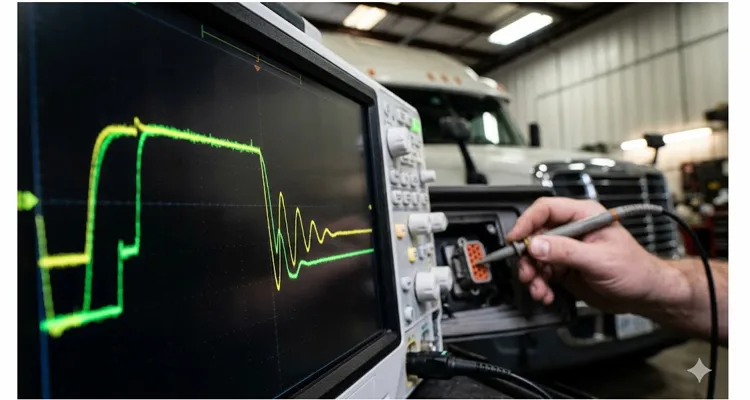
On the Freightliner I mentioned earlier, the dominant-to-recessive edge had a six-hundred-millivolt undershoot that rang three times before settling. That ringing was the reflection from a sixty-centimeter stub returning at exactly the wrong moment. On the scope, it looked like a damped sine wave superimposed on the recessive level — the receiver was trying to decide between a dominant and a recessive bit while the bus was still oscillating. The CAN controller flagged error frames. The ECU stayed silent about it because it never counted enough errors in a row to go bus-off. It just kept retransmitting, every single time. If you want a deeper dive into what those waveform anomalies actually mean, I have written a separate guide on J1939 oscilloscope waveform diagnostics that walks through edge-rate measurements and ringing thresholds in detail.
The same harness also had a half-volt ground offset between the engine block and the cab ECU ground reference, which pushed the common-mode voltage on CAN_L to within three hundred millivolts of the transceiver rail at the remote node. I have covered the fleet-wide cost of exactly this scenario in my article on J1939 ground offset fleet cost — the numbers are sobering. Add alternator ripple from an aging regulator, and the noise margin collapsed to almost nothing. Intermittent transmit errors appeared and disappeared with engine RPM. That half-volt offset was invisible to a standard sixty-ohm resistance check. If you want a step-by-step measurement protocol, refer to my guide on J1939 common-mode voltage shift measurement. The underlying physics of what happens when a CAN bus transceiver is pushed near its common-mode limit is well-documented in semiconductor application notes — but seeing it on a scope in a running truck is a different education entirely.
I have done factory acceptance testing on harnesses where two identically drawn networks, built from the same bill of materials but one with forty-centimeter stubs and another with eighty-centimeter stubs, showed a difference in residual bus error rate of three orders of magnitude — from ten to the minus nine to ten to the minus six. The eighty-centimeter network still “passed” the diagnostic trouble code logic because no node went offline. But in the field, a ten-to-the-minus-six error rate is the difference between a truck that runs a decade without a comm fault and one that visits the shop eight times a year for a problem that never leaves a trace. I have documented how this specific stub length and termination mismatch generates a J1939 bit sampling error that can push a node to bus-off without a single logged DTC.
The Five-Thousand-Dollar Math
Let me put real numbers on this. What follows comes from my own field service logs, warranty analysis from two different Tier-1 suppliers, and maintenance records shared by fleet managers I work with. I write the amounts out in full because there should be no mistaking the scale.
Scenario: a mixed fleet of fifty Class 8 trucks and refrigerated trailers, average age four years, operating regional routes.
- Intermittent comm-loss events per vehicle per year that never mature into hard fault codes: roughly eight to fourteen.
- Average diagnostic time per event across all shops: one-point-seven hours. At one hundred twenty dollars per hour, that is two hundred and four dollars in diagnostic labor per event.
- Average parts replaced unnecessarily per event: three hundred and ten dollars. I keep a folder of photographs of perfectly functional NOx sensors pulled off trucks because they happened to be the module that stopped communicating first during a CAN bus lock-up.
- Vehicle downtime per event: roughly four hours, at a conservative opportunity cost of one hundred dollars per hour. That is four hundred dollars per event.
With eight events per year, the tally per vehicle is: one thousand six hundred thirty-two dollars in diagnostic labor, two thousand four hundred eighty dollars in misdirected parts, and three thousand two hundred dollars in downtime — seven thousand three hundred twelve dollars total. Cut that in half for a fleet with sharp technicians who catch a few before the parts cannon fires, and you are still at three thousand six hundred fifty-six dollars per vehicle. Across fifty trucks, that is one hundred eighty-two thousand eight hundred dollars annually.
That is more than the fully-loaded annual cost of two senior diagnostic technicians — salaries, benefits, tooling, and training. Instead of chasing phantom costs, those two people could be doing productive preventive maintenance that actually extends vehicle life. The money is not being saved; it is being burned on the wrong problem. I have broken down the J1939 physical layer ROI with basic tools elsewhere — fleets that invest in a basic scope and a CAN interface routinely cut diagnostic downtime by more than half.
How I Find What the Standard Procedure Misses
When I walk into a depot to investigate a truck with no codes and a bad attitude, the textbook says: measure termination resistance, check for shorts to ground, verify DC bias voltage, scope the bus. You already know those steps. I do them too — but I do them differently, because I have learned that a standard sixty-ohm reading can lie. Here is the procedure I actually follow, and the parts of it that have saved me more times than I can count.
The Double Measurement
I measure termination resistance twice: once at the diagnostic connector with everything cold, and once with the connector body under gentle side-load. I have watched a sixty-point-one-ohm reading become forty-eight ohms the moment I wiggled the connector shell, because the ECU terminator had a fractured solder joint that opened under mechanical strain. A standard static measurement declared the network healthy. The truck had been in and out of three shops. This is why I always recommend measuring J1939 termination resistance drift hot vs. cold — thermal cycling reveals fractures that a room-temperature check misses entirely. When I need to access tight spaces behind the dash or around the engine bay for these measurements, a J1939 90-degree right-angle cable saves me from putting mechanical strain on the diagnostic port itself.
The Asymmetric Termination Trap
I disconnect one termination at a time and verify each is one hundred twenty ohms by itself. I have found terminators drifted to one hundred forty-seven ohms from moisture intrusion inside a sealed connector body. The parallel resistance read sixty-three ohms, which “looked close,” but the asymmetry created a standing-wave pattern on the bus that corrupted frames on the far node. A junior tech would have moved on. I have also found a truck where the ECU terminator had failed open entirely, and the sixty ohms at the diagnostic connector came from two aftermarket Y-cable terminators installed at opposite ends of a body-builder harness. The bus was terminated — at the wrong locations — and the eye diagram was ninety percent closed. For the full diagnostic flowchart I use when a sixty-ohm reading doesn’t add up, see my J1939 calibration fault troubleshooting flowchart.
The Leak-to-Ground That a DMM Can Miss
CAN_L to ground on a Paccar measured eighty-seven ohms with the key off. That is not a dead short, but a leakage path. The harness had been pinched between a frame rail and a DEF tank bracket during a retrofit, and the insulation was cold-flowing under clamp pressure. The truck had intermittent J1939 communication failures for fourteen months. A standard pin-to-pin continuity test would never have caught it because the wire was not broken — it was bleeding signal current into the chassis. I have written an entire case study on diagnosing J1939 transceiver failure while still communicating that covers how a partially degraded transceiver can pass a resistance check while corrupting frames under load.
The “Differential Walk-Around”
I connect my scope differentially across CAN_H and CAN_L at the diagnostic connector first, then move node to node by backprobing each ECU connector. I look at the dominant-to-recessive transition on a single frame. A clean bus returns to the recessive level with no ringing, no overshoot beyond half a volt, no stair-step plateaus. If I see ringing that decays over three or four cycles, I know there is a stub-length problem or an impedance discontinuity. If the recessive edge rises slowly, the bus capacitance is too high. I once measured bus capacitance exceeding two hundred picofarads — the design limit was sixty — because a body builder had spliced in fifty feet of untwisted nineteen-gauge wire to add a liftgate control module. The bus still “worked,” but every frame spent extra nanoseconds in the indeterminate region. For a practical guide on catching these edge-rate issues with an affordable setup, take a look at my article on J1939 scope bench edge rates, ringing, and differential voltage.
Bit Timing Verification
If I have access to the ECU flash data, I check the sample point. I have seen modules reflashed with a calibration file from a different vehicle architecture where the sample point was set at sixty percent instead of the seventy-five percent the topology required. The network functioned perfectly on a lab bench with a one-meter backbone, but fell apart on a forty-meter bus with six nodes and temperature variation. No diagnostic trouble code ever pointed to a bit timing mismatch. I have covered the diagnostic approach for this exact scenario in J1939 sampling point diagnostics. The SAE J1939 standards family defines the parameter group numbering and application layer that sits on top of this physical layer — but even the most meticulously defined protocol cannot save a bus whose bit timing has drifted outside the transceiver’s decoding window.
The Error Frame Whisper
A Kvaser, PEAK, or Intrepid CAN interface lets me watch bus load and error frames in real time. On a healthy J1939 network, the error frame counter stays at zero for minutes. If I see even one error frame per second, I know something is systematically damaging frames. One per second does not trigger a fault code on any ECU I know, but over an eight-hour shift it is almost thirty thousand retransmissions. That is thirty thousand chances for a sensor reading to arrive late, an actuator command to be missed, or a fault code to land on the wrong module. If you are new to this technique, my J1939 data link error diagnostic guide walks you through the entire process in about twenty minutes.
Four Field Failures That Pass a 60-Ohm Test
These are the patterns I see repeatedly, in fleet after fleet. Every one of them passed a basic termination resistance check at some point and was declared healthy.
The Third Terminator
I have lost count of how many trucks I have inspected where someone installed a Y-splitter cable with a built-in one-hundred-twenty-ohm resistor, creating a third termination and dropping bus impedance to forty ohms. Differential voltage amplitude collapses below the one-point-five-volt minimum, and the bus becomes acutely sensitive to electrical noise. The truck “worked” in the shop at idle. It failed on the highway with the cooling fan engaged. I have broken down the math on how J1939 backbone design and 60-ohm derate directly causes this failure mode. For diagnosing splitter-related issues, I keep a J1939 9-pin pigtail breakout cable in my kit — it lets me monitor bus traffic while isolating each branch of the Y one at a time without cutting into the harness.
The Untwisted Splice
A vehicle network is not a four-to-twenty-milliamp loop. Twisting is what gives you common-mode noise rejection. I have seen maintenance shops splice in ten feet of red-and-black primary wire to fix a rub-through, creating an antenna that coupled alternator whine directly onto the CAN lines. On the scope, you could see the alternator ripple modulated onto every recessive bit. For a detailed walk-through of how to diagnose and fix this, I recommend my J1939 common-mode voltage diagnose ground offset guide.
The Stub That Grew
ISO 11898-2 says keep stubs below zero-point-three meters at five hundred kilobits per second. Every extra ten centimeters beyond that degrades the signal nonlinearly. I have measured usable eye diagrams at forty centimeters that completely collapsed at seventy. The extra thirty centimeters were a cable extension someone added to make a connector easier to reach during service — a convenience modification that introduced a fleet-wide intermittent fault. I have written a comprehensive J1939 backbone termination and stub length guide that includes the exact measurement tolerances I use on every site visit.
The Cable That Looked Identical
The market is flooded with cables that use copper-clad aluminum conductors with thirty to forty percent higher DC resistance than the spec allows, PVC jackets with no shielding continuity, and gold flash so thin it wears through in twenty mating cycles. Resistance drifts. Capacitance drifts. A network calibrated at assembly degrades two years later not because any component failed, but because the interconnect was never built to stay inside the tolerance band over time and temperature. This is exactly why I documented the J1939 termination and stub length phantom fault cost — the cable is often the last thing anyone suspects, and the first thing that should be checked.If you are responsible for fleet procurement, I have also published a J1939 cable quality TCO guide that breaks down why the cheapest harness consistently costs three times more over its service life once you account for diagnostic hours and unplanned downtime.
Case In Point: The Refrigerated Fleet That Would Not Stay Connected
A cold-chain fleet in the UK was running forty-five tractors with trailer telematics units communicating over CAN via SAE J560 / ISO 12098 seven-pin connections. The telematics units would randomly drop offline for six to twenty seconds, then recover. The refrigeration unit manufacturer blamed the telematics supplier. The telematics supplier blamed the tractor. The fleet owner was ready to replace the entire telematics system at a cost of three hundred forty thousand pounds.
I spent two days on-site. By the end of day one, I had the root cause: the seven-pin coiled cables connecting trailer to tractor had been replaced over time with a cheaper aftermarket cable that deviated from the standard impedance and had a measured electrical length equivalent to a stub of two-point-one meters — four times the maximum allowed at the two-hundred-fifty-kilobit data rate. The eye diagram on the trailer node was fully closed. In the lab, with a one-meter standard cable, the system was flawless. On the road, the long, high-capacitance coiled cable made it intermittent. I have covered this exact failure — where aftermarket parts erode network reliability — in my analysis of J1939 aftermarket telematics cost and network reliability. When retrofitting fleets with mixed connector types, a J1939 9-pin female to DT 12-pin male adapter cable ensures the transition from the diagnostic port to the Deutsch-based trailer harness maintains the correct pin-to-pin continuity and impedance.
The fix was not new telematics units. It was reverting to OEM-spec coiled cables with verified one-hundred-twenty-ohm impedance and a maximum length that respected the stub limit. Cost per vehicle: forty-seven pounds and twenty minutes of labor. The fleet’s phantom disconnects stopped within a week.
How to Verify the Fix Actually Worked
After correcting a network calibration issue, do not accept “the code didn’t come back” as sufficient evidence. Do this:
- Record twenty-four hours of CAN traffic and review the error frame counter. It should be zero or near zero over the entire logging period.
- Perform a mechanical wiggle test with the scope connected — flex every connector, move every harness segment near a heat source or bracket, and watch for differential-voltage anomalies. I have published a complete wiggle test protocol for J1939 harness opens that covers the exact procedure, including what voltage deviations to consider a fail. For a broader guide on catching intermittent faults, see my article on intermittent J1939 faults with the wiggle test.
- Run a worst-case bus load test — activate every ECU that transmits periodically, cycle high-current loads like cooling fans and grid heaters, and verify bus load never exceeds the design threshold.
- Thermally cycle the vehicle — park it outside in ambient overnight, then run to full operating temperature while logging. I have caught calibration drift that only appeared below minus ten Celsius or above eighty Celsius.
- Document the before-and-after resistance, capacitance, and waveform measurements. If the problem ever resurfaces, that baseline is your single most valuable diagnostic tool. For guidance on deciding whether to invest in your own diagnostic setup, my fleet oscilloscope cost-benefit decision guide walks through the math.
FAQ: Questions Engineers and Fleet Managers Ask Me
Q1: Can a network calibration fault cause derate or limp mode without any DTC?
Yes. I have documented multiple cases where an engine ECU stopped receiving valid torque request messages from the accelerator pedal module due to repeated CAN frame loss. The ECU did not log a network fault — it simply executed its substitute value routine and limited torque. The vehicle felt sluggish. No MIL. Only a CAN trace revealed the missing pedal messages.
Q2: Why do these faults seem more common on newer trucks?
Newer vehicles carry more ECUs — twenty to thirty-five nodes is now common — and higher bus utilization from ADAS, telematics, and diagnostics. I pulled the bus load data from a 2012 Cascadia and a 2024 Cascadia running the same route, same trailer, same driver. The 2024 averaged forty-two percent bus load at highway speed; the 2012 averaged nineteen percent. That margin erosion is invisible to the driver, but it means far less time is available for retransmissions when something degrades. For a full breakdown of what happens when a J1939 backbone design fails under elevated bus load, I have covered the physics in detail.
Q3: Does CAN FD make network calibration more or less critical?
More critical. CAN FD transmits the data phase at up to eight megabits per second with a bit time as short as one hundred twenty-five nanoseconds. The allowable stub length at that speed is virtually zero for a passive-star topology. Impedance control, connector quality, and termination precision become non-negotiable. A connector that was “good enough” for five hundred kilobits per second may be completely inadequate for CAN FD.
Q4: What tools do I need to diagnose this myself?
At minimum: a two-channel oscilloscope with at least one hundred megahertz bandwidth, a good DMM with capacitance measurement, and a CAN-to-USB interface with software that counts error frames. I carry a battery-powered isolated scope because I have been burned by ground loops introduced by bench instruments. A full network analyzer like a Vector CANscope is ideal but not necessary for field work. I have written a detailed J1939 waveform analysis guide using a 200-dollar USB scope that proves you do not need a five-figure budget to get started.
Q5: Can poor-quality OBD extension cables or breakout adapters cause network calibration faults?
No — but not for the reason you might think. It is not the cable’s DC resistance that hurts you most. It is the connector barrel capacitance that adds five to eight picofarads per breakout, and that is enough to tilt the bit timing window if your network is already operating near the edge. I have evaluated dozens of aftermarket breakout adapters, and the worst ones add enough lumped capacitance to measurably slow the recessive-to-dominant edge. If you use a breakout box for diagnostics, remember: its electrical characteristics become part of the network for as long as it is connected.
Q6: How often should I proactively check network health?
For mixed-mission fleets with frequent body builder modifications, I recommend a network impedance and waveform check at every major PM interval — or at minimum, annually. The check adds twenty minutes to a PM and can prevent thousands of dollars in random fault code diagnosis. I have one fleet customer who made this a standard PM line item and cut their annual diagnostic hours by more than thirty percent in the first year. The J1939 physical layer troubleshooting 60-ohm waveform guide covers the exact checklist I use.
Q7: Does LIN bus have calibration problems too?
Yes, though they manifest differently. A LIN bus relies on a pull-up resistor at the master, typically one kilo-ohm, and a single wire plus ground. If the pull-up drifts or the total bus capacitance exceeds the LIN specification — often from too many slave nodes or excessively long wiring runs — the rising edge slows down and slave response errors occur. I have seen a LIN bus on a seat control module that failed only when the cabin temperature exceeded forty-five degrees Celsius, because the pull-up resistor’s temperature coefficient shifted it outside the timing budget.
Q8: Are network calibration faults covered by standard diagnostic tooling?
Partially. A modern OEM scan tool can show you message timeout counts or inactive DTCs buried in fault memory. But the resolution is coarse — you see that a message was lost, not why. For root cause, you need an oscilloscope and a protocol analyzer. I tell technicians: the scan tool tells you what fell off; the scope tells you why it tripped. This is exactly the argument I make in my CAN bus physical layer test saving eight hundred dollars in diagnostic fees case study.
Q9: Can temperature extremes physically alter the calibration of a fixed network?
Yes. Cable dielectric constant changes with temperature, which alters capacitance per meter. Termination resistor values drift with temperature coefficient — typically fifty to one hundred parts per million per degree Celsius for thin-film, more for carbon composition. A network calibrated at twenty degrees Celsius can be measurably different at minus thirty or plus eighty-five. I have caught intermittent faults that only appeared after cold-soak because the combined impedance shift moved the sample point just enough to cause occasional bit errors. The connection between a minuscule 0.3V ground offset and J1939 backbone cost is one of the most overlooked root causes in cold-weather diagnostics.
Q10: How do I know if my current supplier’s cables and connectors are contributing to the problem?
Ask for the impedance plot, a TDR test report, or at minimum a documented capacitance-per-meter and resistance-per-meter specification with tolerance bands over temperature. If the supplier cannot provide these, or if their measured variation exceeds your network design margin, the cables are a latent defect waiting to mature into an intermittent fault. I have disqualified multiple cable sources this way — not because they were dishonest, but because they had never been asked to characterize their product at the level a high-speed network demands. For guidance on selecting connectors that maintain signal integrity, I have written about Deutsch connector series selection and maintenance budget impact as well as a dedicated J1939 Deutsch DT and HD connector guide.
A Note on Engineering Support
If you have read this far, you are probably the person inside your organization who gets handed the problems nobody else can solve — the ones with no clear fault code, no TSB, and no flowchart. I have been on the factory floor of a cable and harness manufacturer for over twenty years, and I can tell you that the difference between a cable that holds a network calibration for a decade and one that drifts out of spec in eighteen months is invisible to the naked eye.
Let me give you an example. During a routine insulation-resistance test on a production batch — step three of our quality process — one cable flagged a reading that was within the pass limit but ten percent lower than its neighbors. Under magnification, we found a single strand of copper whisker that had pierced the XLPE jacket during stripping. In the field, that would have created an intermittent short to ground that only appeared when the harness flexed during cornering. The cable would have passed a continuity test and a visual inspection. It would have been shipped. It would have caused a ghost fault six months later that no scan tool could find. That single catch is what a four-step quality inspection actually means — not a checklist, but a series of gates designed to catch the failure modes that only appear under mechanical and thermal stress.
Our facility operates under 5S methodology with climate-controlled storage specifically to protect raw cable dielectric properties from humidity and temperature cycling. All plastic components are RoHS-compliant, full-plastic overmold or mechanical assembly — no secondary painting that can flake and contaminate contacts. Every assembly is 100% tested before it leaves the floor. We hold ISO 14001 certification for environmental management across our production processes, and our IATF 16949 certification validates that our quality management system meets the most stringent automotive requirements. These are not decorations on a wall; they are the framework that makes repeatable quality possible across thousands of units.
We provide OEM customization — logo, branding, cable length, jacket color, conductor AWG — and we work directly with engineering teams who need a supplier that can read a customer-specific drawing, challenge a tolerance if it conflicts with network physics, and deliver a part that matches the specification exactly, batch after batch.
If you are diagnosing a persistent network problem that you suspect has a physical-layer root cause, or if you are specifying cables for a new vehicle program and you do not want to inherit someone else’s calibration headache, reach out.
Contact our engineering team directly:
- WhatsApp: Chat with Linda on WhatsApp
- Contact Page: https://obd-cable.com/contact/
No sales scripts. No automated chat bots. Just engineers talking to engineers. Send us your bus topology, your current waveform captures, or your mechanical constraints, and we will help you determine whether a network calibration problem is at the root of your fleet’s phantom costs — and what the right interconnect solution looks like.
