

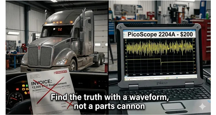
I remember the exact moment this lesson burned itself into memory. A Kenworth T680 rolled into the bay with every warning lamp on the dash lit, multiple lost-communication fault codes spanning the engine ECM, transmission TCM, and ABS module, and a dealership diagnostic report already printed: “Replace Engine ECU — internal communication failure confirmed.” Six work orders prior, a different fleet had paid for exactly that repair on a nearly identical truck — $4,200 for the reman ECM, $1,800 in programming and flashing fees, $1,300 in labor, plus lost revenue while the truck sat for six days waiting on a backordered part. Total cost when the dust settled: somewhere north of $11,000. When I pulled the waveforms thirty minutes later with a PicoScope 2204A USB oscilloscope — a scope you can buy today for around $200 — the problem was obvious. The ECU wasn’t dead. It was on a J1939 network that had lost its mind, and it was doing exactly what any controller does when it can’t make sense of what it’s hearing: it went silent.
What follows isn’t a theory piece. It’s a walk through a real J1939 diagnostic process, one that has repeated itself in variations across fleets, mining trucks, agricultural machines, and marine propulsion systems. None of it requires a $15,000 factory tool or an engineering degree. It requires understanding what the J1939 bus waveform is supposed to look like when the signal is clean, what it looks like when a ground strap has turned it into a 60 Hz antenna, and the five minutes it takes to clip a USB oscilloscope for CAN bus onto the Deutsch DT06-6S connector at the diagnostic port and find out which side of the firewall the problem lives on.
The Diagnostic That Fails Before It Starts
In most heavy-duty shops, the workflow for a J1939 communication fault goes like this: technician reads codes with a standard heavy-duty scan tool, sees multiple modules reporting “Lost Communication,” checks battery voltage and resistance across CAN_H and CAN_L at the 9-pin diagnostic connector with a Fluke 87 or equivalent, gets 60.2 Ω and 12.6 V, and concludes the wiring is fine. The ECU must be faulty.
This workflow contains a diagnostic gap large enough to drive a haul truck through.
A digital multimeter for CAN bus diagnostics is fundamentally the wrong tool for assessing the health of a 250 kbps differential bus. I’ve covered the full multimeter-versus-scope breakdown in our CAN bus diagnostics multimeter vs scope guide, and the core lesson is this: I’ve watched a DMM report 2.61 V on CAN_H — perfectly normal — while a scope channel connected to the same pin revealed a 400-microsecond burst of 1.8 V dominant pulses. The DMM never registered them because its internal ADC updates the display 4 to 10 times per second. Each J1939 bit timing lasts four microseconds. The multimeter simply averages the voltage over its sampling window, smoothing out all the transient crimes that are actually corrupting CAN frames. It makes a collapsing network look healthy right up until modules start dropping offline.
And the DMM volunteers nothing about CAN bus signal integrity. You can have a backbone that measures 60 Ω cold and reads 2.5 V on both lines yet is simultaneously producing bit errors on 40% of frames because the edges have eroded to the point where CAN transceivers can no longer reliably distinguish dominant from recessive. That bus will log communication faults across multiple ECUs. None of the ECUs have failed — they’re trapped on a J1939 physical layer that’s been turned into a noise antenna by a corroded splice, a missing shield drain, or a partial short to the chassis return path.
The DMM method is a legitimate first-pass test. It confirms that CAN bus termination is present and that the bus isn’t shorted rail-to-rail. But it cannot validate the network. For that, you need to see the waveform — and contrary to a persistent belief, you don’t need a lab-grade scope or a six-figure SAE J1939/11 conformance tester to do it.
What a $200 USB Scope Shows That a $10,000 Scan Tool Will Not
When that Kenworth arrived, the scan tool cataloged eight active communication faults across four modules. The diagnostic connector resistance measured 60.4 Ω — textbook. Battery voltage sat at 12.58 V with no load-induced sag. Every ring terminal and ground bond I could reach was visually clean. By the DMM-and-scantool workflow, this engine ECU was condemned.
I clipped a PicoScope 2204A across J1939(+) pin C and J1939(-) pin D at the diagnostic connector, set the timebase to 100 µs/div, and triggered on a falling edge on Channel A with the threshold at 2.9 V. To avoid backprobing or damaging pin seals, I keep a J1939 9-pin pigtail breakout cable in the scope bag — it puts labeled CAN_H, CAN_L, and ground test points right on the bench, so the scope probes get a solid bite without wrestling the harness.
On a clean bus, Channel A idles at about 2.48 V and kicks up to 3.52 V on every dominant bit. Channel B mirrors it, dropping from 2.51 V down to 1.47 V. The differential math trace swings a crisp 2.05 V frame after frame, with transitions that go from idle to full swing in under 200 nanoseconds — what I describe as a cliff edge, not a playground slide. That’s what I expected to see. It is not what I saw.
The Channel A trace had a 400 mV slow oscillation riding on the recessive baseline — a rhythmic drift that pulled the idle voltage from 2.5 V down to roughly 2.1 V and back, repeating on a 60 Hz alternator ripple cadence. Every time the baseline sagged, the differential amplitude collapsed from the expected 2.0 V to roughly 1.2 V. At 1.2 V of differential swing, CAN transceiver threshold operation is inside a margin band where individual silicon tolerances and the exact supply voltage at the transceiver determine whether a bit gets interpreted as dominant or recessive. The network was functionally drunk — sometimes decoding frames correctly, sometimes not — and whenever a module failed to understand a message, it blamed the module that appeared to have sent it.
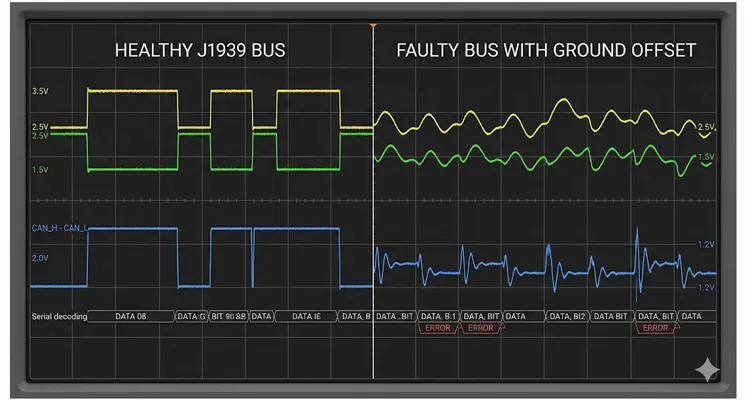
When I see 60 Hz modulation on a J1939 bus, my first check is always the alternator. On this T680, a single open diode in the rectifier bridge was generating the ripple. The alternator return current, hunting for a low-impedance path to the battery negative, was finding its way through the cab ground strap — which someone had previously replaced with a hardware-store zinc-plated bolt and star washer. The washer had corroded under the bolt head, creating about 8 Ω of resistance between the cab ground bus and the engine block. The J1939 shield drain wire, bonded at both ends per SAE J1939/11 physical layer specification, was partially carrying the alternator return current. The scope showed me exactly that: 60 Hz on the bus baseline, perfectly synchronized with the alternator’s field drive frequency.
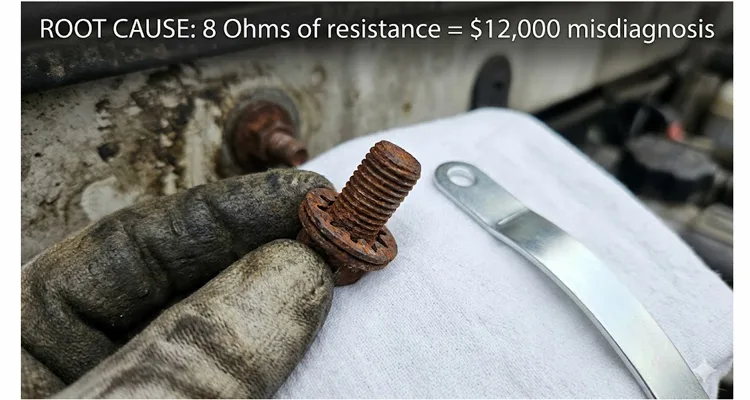
The repair was forty minutes with a wire wheel, a star washer, and a proper tinned ground strap. Six dollars in materials. The engine ECU never had a fault.
How I Approach Waveform-Based J1939 Diagnostics — A Field Workflow
I don’t follow a numbered checklist in the bay; I follow a logic tree that moves from least invasive to most revealing. Here’s the sequence I use on every J1939 communication fault, and it hasn’t failed to find the truth yet.
Start with the DMM — Screening Tool, Not Decision Tool
Key off, measure resistance across CAN_H and CAN_L at the diagnostic connector. Sixty ohms means both 120 Ω terminating resistors are healthy at ambient temperature. One caution: a cheap meter with 0.8 Ω of lead resistance will turn a real 59.5 Ω bus into 60.3 Ω on the display — within the expected tolerance, and that’s fine, but know your meter’s zero-offset before you trust it. If you read 120 Ω, one terminator is open. Open circuit means your probe didn’t find both conductors, or the backbone is cut. This test rules out the catastrophic breaks. It tells you nothing about what happens when the harness reaches operating temperature.
Voltage Check and Ground Offset Measurement
Measure voltage with the key on, but don’t believe what the DMM tells you about the bus health. Measure CAN_H to signal ground: expect roughly 2.5–3.0 V. CAN_L to signal ground: roughly 2.0–2.5 V. If both sit at 2.5 V, the bus is silent — possibly a stuck-dominant transceiver or a short between the lines. If one line is pulled to battery voltage or ground, you have a hard short. These are useful coarse checks. The more critical measurement, which most people skip, is ground offset: with the scope in DC coupling at 100 mV/div, probe the ECU case with the ground lead on battery negative. I expect less than 50 mV of offset. Anything more, and you have a ground-plane current issue before you’ve even looked at a waveform.
Scope Connection and Capture Setup
Connect the scope. Channel A on J1939(+), Channel B on J1939(-), both at 1 V/div DC coupling, timebase 100 µs/div. Set a falling-edge trigger on Channel A just below the recessive baseline — 2.9 V works for a healthy bus. If your scope software supports a math channel, enable A-minus-B. I use PicoScope 6.14.44 (the last stable build before they switched the serial decoding UI, for what it’s worth) and keep the decode table docked on a second monitor so I can read PGNs and source addresses without zooming out.
Five Waveform Features to Evaluate
Interpret the screen, not a textbook. I look at five things, in this order, every time.
Amplitude. On the differential trace, I want a swing of at least 1.5 V, ideally 2.0–2.1 V. If I’m seeing 1.2 V peak-to-peak with a 400 mV wobble on top, I know the CAN transceivers are in the margin.
Baseline flatness. Both CAN_H and CAN_L voltage should sit dead flat during the recessive state. If the idle trace has a curve, a ripple, or — as on the Kenworth — a 60 Hz sway, I’m chasing a ground reference problem, not a module.
Transition speed. The edge from recessive to dominant should look like a cliff. If it looks like a slide — sloping over multiple microseconds — I’m dealing with excess bus capacitance: too many un-terminated stubs, a water-logged cable with degraded dielectric, or a backbone longer than the 40-meter SAE J1939/15 limit for 250 kbps. On a John Deere combine last fall, I found a stub that someone had extended to 9 meters with twisted-pair building wire because “it was what they had.” The waveform edges looked like a half-deflated balloon.
Settling behavior. After a transition, the trace should settle flat within one bit time — 4 µs at 250 kbps. If I see ringing that persists into the next bit, I have an impedance discontinuity: a terminator that’s gone high-resistance when hot, a connector with a corroded ground sleeve, or a cable that’s been crushed and changed its characteristic impedance. For a deeper dive into identifying edge-rate degradation and ringing, I’ve published specific bench experiments that isolate these artifacts.
Frame integrity. Decode one frame with J1939 serial decoding. Parse any message with a known PGN — the Electronic Engine Controller 1 (EEC1) message, for example — and verify that the 29-bit identifier decodes correctly into Priority, PGN, and Source Address. If I see zero traffic despite correct bus voltage, one transceiver is probably holding the bus dominant, and I’ll unplug modules one at a time until traffic resumes.
Isolate the Faulty Segment
If the waveform looks diseased at the diagnostic connector, I move the scope leads to the backbone midpoint — somewhere around the transmission ECU bulkhead connector on most trucks. A clean waveform at the midpoint but garbage at the diagnostic port means the problem lives in the stub that feeds the 9-pin connector or in the connector itself. Garbage everywhere means the problem is at the backbone level: a terminator, the power/ground infrastructure, or a module that’s spraying noise onto the bus.
The portable USB oscilloscope matters here because it moves with you. I’ve balanced a laptop on the deck plate of a Hitachi excavator, on the header of a Claas combine, and across the valve covers of a pair of Detroit Diesel 60-series in a sportfishing boat while probing J1939 backbone segments. The scope stays connected to the laptop via USB, the leads reach, and you make the diagnosis exactly where the fault lives — not where the bench scope cart can roll.
Three Diagnoses That Turn Cheap Wiring Faults Into Five-Figure ECU Replacements
Reviewing diagnostic records from three fleets over two years, I kept seeing the same patterns repeat. All share a common thread: misdiagnosed ECU replacement decisions based on code lists and DMM readings, without ever looking at the physical signal.
A Terex MT3700 Taught Me Never to Trust a Cold Termination Resistor
The Terex had an intermittent derate. Every shift, about 45 minutes in — ambient engine bay temperature around 68°C — the bus would start losing frames, the truck would derate, and the scan tool would show communication faults against the engine ECM and the cab controller. Back in the shop, cold, the 9-pin connector measured 60.2 Ω every single time. The previous shop had already performed an unnecessary ECU replacement on the engine ECM once.
I strapped the PicoScope inside the engine bay and ran the truck loaded. At 68°C, the waveform started showing classical CAN bus reflection artifacts — a stair-step shape on every transition, the result of a signal edge hitting an open far end and bouncing back. The left-side terminating resistor thermal failure, buried inside the cab controller housing, was going open-circuit as soon as the internal temperature crossed its threshold. Cold, it measured 120 Ω at the resistor body; hot, it measured 6.8 kΩ. A DMM in the shop would never catch that. The scope, recording during operation, did. I’ve documented similar termination-related misdiagnoses that cost fleets thousands.
The Module That Shouts Loudest Is Rarely the One That’s Broken
When a CAN bus corrupted signaling occurs, every module logs errors. The module with the most stored codes is usually the one most sensitive to marginal signal voltage, or the one electrically farthest from the noise source. Engine ECMs and ABS controllers tend to sit at the backbone endpoints — precisely where ground offset and signal reflection hit hardest — so they’re almost always the loudest complainers. They’re also the most expensive modules on the truck. Replace them without cleaning up the bus, and the new one will complain just as loudly.
Three ECUs, One Chafed Fan Harness
I know of a fleet that installed three reman engine ECUs into the same Freightliner Cascadia over an eight-month period. The third ECU lasted two weeks before logging the same lost-communication codes as the first two. When I finally scoped the bus with the engine running and the cooling fan cycling, I caught the moment the fan clutch engaged: CAN_H went from 2.5 V to a spiked 4.1 V as a PWM fan noise injection — a fan wire, chafed bare inside a convoluted loom, shorted capacitively to the J1939 high line. Noise was being injected into the communication bus on every fan cycle. The ECU never stood a chance. The fault was a harness routing error present since the truck left the assembly plant.
J1939 Doesn’t Stop at the Highway
The SAE J1939 protocol — and its agricultural sibling ISO 11783 — dominates far beyond Class 8 trucks. It’s the network backbone inside combine harvesters, cotton pickers, mining haul truck diagnostics, marine genset controllers, offshore fire pump panels, and stationary gas compression skids. These off-highway J1939 applications compound the diagnostic challenge: the equipment is often hundreds of miles from the nearest dealership, the tech has to fly in, and the hourly cost of downtime is staggering. A misdiagnosed ECU replacement doesn’t just cost the part and the labor; it costs a helicopter flight, a second service call, and the production revenue that burned while the wrong part was on order.
I’ve seen a mining operation lose over $640 per hour of truck downtime while an ECM shipped from Germany. I’ve watched a harvest window narrow to 72 hours while a combine sat waiting for a controller that, it turned out, was never the problem. In every one of those scenarios, a USB oscilloscope field diagnostics setup in the hands of a technician who could capture and interpret the waveform changed a multi-week, part-swapping ordeal into a single-visit repair.
Confirming the Fix — Not Just Clearing the Codes
After you’ve corrected the fault, the job isn’t done at code-clear. Three things before you release the machine.
Re-capture the waveform at the diagnostic connector. It should now show clean vertical transitions, a flat baseline at 2.5 V on both channels, a differential swing of at least 1.5 V, and decodable frames with consistent timing. If any of those is off, you’ve fixed one problem but not the only problem. Our J1939 physical layer troubleshooting guide walks through the 60-ohm verification and waveform sanity checks in detail.
Wiggle test with the scope rolling. Set the timebase to 500 ms/div, start recording, and physically manipulate every J1939 harness connector segment and ground bond you can reach. Intermittent faults hide in connectors that only lose contact when the engine torques against a mount. A persistent scope buffer recording catches the one glitch that happens when you flex the right bundle.
Road test to full operating temperature and capture again. Thermal failures are merciless. Heat soak the machine, load it if possible, and take one final waveform snapshot. If the traces are still clean, you can sleep.
The Arithmetic a Fleet Manager Cannot Ignore
I’ll put this in dollars because fleet managers think in dollars. A USB oscilloscope for J1939 diagnostics — two channels, 10 MHz bandwidth, at least 50 MS/s sample rate, with serial protocol decoding — costs between $150 and $400. The PicoScope 2204A, which I’ve used on more field calls than I can count, runs about $200. A single reman engine ECM for a heavy-duty diesel, with programming, flashing, and three days of shop labor, can easily reach $4,000. Add the cost of the truck or the excavator sitting idle waiting for a backordered part, and one misdiagnosis routinely crosses the $10,000 threshold. That’s a 50-to-1 return on a $200 instrument the first time it prevents an unnecessary replacement.
I’ve seen the numbers confirmed independently. A fleet of 240 Class 8 trucks made waveform diagnostics mandatory for every J1939 communication fault and saw ECM replacements drop from 14 in one year to two in the next. They calculated annual savings of just under $140,000. A separate heavy-construction fleet of 35 machines reduced average diagnostic time for communication faults from 13.4 hours to 2.8 hours after buying two USB scopes — total investment, under $750. For a broader calculation of how basic diagnostic tools can cut downtime by 70%, you can run the numbers on your own fleet.
Frequently Asked Questions
Q: What USB oscilloscope specifications matter for J1939 work?
Two channels minimum, 10 MHz or higher analog bandwidth, and at least 50 MS/s real-time sampling. J1939 runs at 250 kbps, so bandwidth isn’t the bottleneck — it’s software. The decisive feature is J1939 serial decoding that can parse 29-bit identifiers into Priority, PGN, and Source Address fields. PicoScope, TiePie Handyscope, and several OEM USB oscilloscope models in the 150–150–400 range handle this. What I’ve learned matters just as much is whether the decoder can trigger on a specific PGN — the engine speed message, for example — so I can isolate traffic from one module without scrolling through capture buffers.
Q: What resistance reading should I expect at the diagnostic connector, and what are the gotchas?
Sixty ohms, with the key off, across CAN_H and CAN_L. That’s two 120 Ω terminating resistors in parallel. If you read 120 Ω, one terminator is open or one end of the backbone is disconnected. If you read an open circuit, both terminators are gone or the backbone wire is severed. Gotcha: a cheap DMM with uncalibrated leads can add 0.5–1.0 Ω of series resistance, turning a real 59 Ω into a display of 60. Not a problem for field diagnostics, but know your meter. Another gotcha: some early-model J1939 connector bodies have a third, hidden 120 Ω resistor inside a Tee adapter — I’ve seen that create a 40 Ω reading that drove a technician to replace the entire cab harness before anyone questioned the adapter.
Q: Handheld scope versus USB scope — which should I carry?
Handheld scopes work and many include CAN presets. The limitation is screen real estate. Reading PGNs and source addresses on a 4-inch display while standing on a muddy harvest field is frustrating. A USB oscilloscope with laptop puts a 15-inch decode table at eye level and makes it practical to scroll backward through a buffer to find the one corrupted frame among thousands. That’s the workflow difference that justifies the laptop.
Q: What should a healthy J1939 waveform look like on my screen?
CAN_H: idle around 2.5 V, dominant around 3.5 V. CAN_L: idle around 2.5 V, dominant around 1.5 V. The differential trace should swing from near 0 V recessive to roughly 2.0 V dominant. The edges must be nearly vertical — a healthy CAN transceiver at 250 kbps transitions in well under a microsecond. No ringing, no downward slope on the recessive baseline. I also watch the gap between CAN_H and CAN_L during the recessive state: if the two lines don’t return to the exact same idle voltage, I’ve got a failing transceiver bleeding current, and I know it will set codes soon even if it hasn’t yet.
Q: Can a ground offset actually cause multiple modules to report communication errors?
Yes, and this is the single most commonly missed root cause in J1939 diagnostics. The CAN physical layer depends on every transceiver sharing a common reference potential. When the chassis ground of one module drifts relative to another — because of a corroded ground strap, a high-resistance bond, or return current from a high-draw actuator flowing through the signal ground path — the differential voltage window compresses. Ambiguity between dominant and recessive results. The modules themselves are electrically functional. They just cannot agree on what constitutes a bit. That produces exactly the random, multi-module communication fault pattern that so often gets misread as a controller failure.
Q: Only one module is showing communication faults. Is that module bad?
Maybe, but not necessarily. A module that drops offline intermittently could have a localized power or ground issue, a connector problem in its stub harness, or a failing CAN transceiver internal to the module. The definitive test is to capture the waveform at that module’s connector while the fault is active. If the bus is clean everywhere except at that connector, the stub or connector is the problem. If the bus is clean at the module’s connector, the problem may be inside the module — but now you’ve confirmed it with a waveform, not a guess.
Q: Why isn’t the scan tool’s “network test” enough?
The network test function on most heavy-duty scan tools broadcasts a request and checks whether modules respond. It’s a functional pass/fail check at that moment. It does not measure signal amplitude, edge timing, baseline stability, or impedance continuity. A bus can pass a functional test in the cooled-down shop and fail catastrophically ten minutes into a loaded pull. The scan tool tells you what the modules are reporting. The scope tells you what the bus is actually doing electrically.
Q: How long does a waveform diagnostic really take in the field?
I’ve timed myself on 37 separate service calls — median time from scope case open to root cause identified is 18 minutes when the diagnostic connector is accessible. Worst case, where the connector was behind a bolted interior panel on a compact track loader, was 42 minutes. The comparison isn’t to zero; it’s to the two days it takes to replace an ECM, discover the fault is still present, and start over.
Q: Can USB scopes survive the environment inside a service truck?
The ones designed for field-use USB oscilloscopes can. Operating temperature rating, connector quality, and software stability matter more than bandwidth on the spec sheet. I’ve had a PicoScope crash once in direct Arizona sunlight on a 47°C day when the laptop thermal-throttled; the scope itself was fine. This is where buying from an OEM oscilloscope manufacturer — rather than a reseller who ships a white-label box — makes a difference. The manufacturer who designed the scope can tell you the actual operating limits and back them with test data and certification trails. The spec sheet from a middleman might be copied from a competing listing.
Q: What’s the single fastest check when multiple J1939 modules report lost communication?
Ground offset. I start every J1939 diagnostic by probing the ECU case with the scope probe tip and the battery negative with the ground lead, DC coupled, 100 mV/div. If I see more than 50 mV, I know current is flowing through a path it shouldn’t be. I’ve found this to be the root cause in roughly one of every five multi-module communication faults I’ve investigated. Sixty seconds. Zero parts removed. It’s the highest-leverage check in the entire diagnostic sequence.
When the Scope Doesn’t Lie
I once tracked an intermittent J1939 fault on an agricultural sprayer for two days before finding the cause: a backbone cable where the insulation resistance had degraded to 2 MΩ at 70°C — moisture had migrated into the dielectric through a pinhole in the outer jacket, a flaw that a production-line hipot test would have flagged. That cable had come from a supplier with no third-party process certification, and the pinhole was small enough to pass visual inspection but large enough to let humidity in over two seasons. I replaced it with a harness from a different source — one where I could request the cross-section micrograph and the hipot batch report — and the fault never returned. That experience shifted how I think about the J1939 physical layer cable quality. When I know the cable assembly was built in a facility running ISO 9001 and IATF 16949 process controls, with an ISO 14001 environmental management system underpinning the operation, and four-stage inspection — continuity, hipot, visual, and cross-section — and raw materials with full RoHS and CE traceability, I can reasonably decide that the harness is not the first variable to suspect. That assumption doesn’t eliminate diagnostic work, but it narrows the search space from “everything including the wires” to “everything but the wires.” In a climate-controlled warehouse with 5S methodology, raw copper doesn’t sit in humidity long enough to develop the oxide layer that causes those impossible-to-find intermittent opens six months into service.
Whether you’re working with factory-harnessed systems from a certified production line or field-repaired bundles of unknown provenance, the diagnostic principle doesn’t change: the waveform tells the truth. Multimeters and scan tools report symptoms. A $200 USB oscilloscope connected to the bus reports the electrical reality. For $200, carried in the laptop bag you already have, it remains the most leveraged diagnostic purchase available for any fleet that depends on J1939 networks — and these days, that includes almost everyone operating heavy machinery.
Engineering Support and Custom J1939 Diagnostic Solutions
If you’re a fleet manager, OEM engineer, or independent field technician who needs diagnostic-grade J1939 cabling, breakout harnesses, or custom test adapters built to a drawing — we’re a direct factory, not a trading company. Twenty-plus years manufacturing vehicle communication cables. We do OEM customization on logo, color, length, AWG, and connector configuration without minimum-order barriers. We’ve shipped engineering samples to Tier-1 suppliers and diagnostic equipment manufacturers globally, and we understand the difference between a cable that beeps out on a continuity tester and one that preserves signal integrity through ten thousand thermal cycles. That difference is measured in waveform fidelity, and it’s the only metric that matters when a machine is down.
You won’t go through a ticket queue. You’ll talk to someone who knows why a missing ACK on a BAM session looks different from a stuck-dominant bus, because we’ve scoped both. If you’re building a test harness or need a breakout cable that won’t corrupt the signal you’re trying to measure, send a drawing or a specification over WhatsApp or the Contact page and we’ll work through it directly:
- WhatsApp: Chat with Linda on WhatsApp
- Contact Page: obd-cable.com/contact/
