

A factory engineer’s perspective on why the cheapest diagnostic tools often deliver the highest return
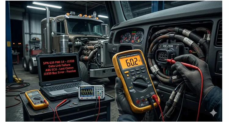
During a third-shift line-down call last winter, I traced a 72-hour telematics outage back to a single strand of copper that had fatigued under a cable tie. The diagnostic laptop said “ABS ECU Timeout.” The Fluke 87V said “4.7 kΩ on CAN-H.” That gap in information — between what the scan tool reports and what the wire actually carries — is where fleets hemorrhage 70% of their diagnostic labor budget.
I’m talking about the physical layer. The copper. The connectors. The 60 ohms you’re supposed to see between CAN_H and CAN_L but never actually verify because “it worked yesterday.” The twisted pair that’s been pinched behind a bracket for six months, slowly fretting its way toward an intermittent open.
When we talk about J1939 network failures in heavy equipment, the conversation almost always starts at the wrong layer. Someone pulls a laptop, launches diagnostic software, and starts hunting for SPN 639 FMI 14 — the infamous J1939 Data Link Failure code. They see a dozen modules all throwing “lost communication” faults, and the natural instinct is to suspect the module that’s screaming loudest. I’ve watched competent technicians spend three days chasing phantom ECU failures when the actual problem was a 15-minute termination resistor check they never performed.
This isn’t a criticism. It’s a reality of how we’re trained. We trust the software. We trust the scan tools. We forget that none of it matters if the underlying electrical path is compromised. If you’re staring at a screen full of SPN 639 faults and haven’t yet reached for a multimeter, you’re about to lose money. We’ve covered the exact diagnostic sequence that replaces guesswork with verification in our J1939 data link error diagnosis guide.
The cost math nobody wants to talk about
Let me put some numbers on this. Heavy equipment downtime in mining or construction applications runs anywhere from $500 to $3,000 per hour depending on the asset. A Kenworth T680 sidelined by a CAN network failure can cost a fleet $2,500 per day in lost revenue before you even touch the repair bill. When network faults cascade across multiple vehicles — and they do — the financial impact compounds rapidly. Even if we anchor to the conservative floor of that estimate, a fleet experiencing just three physical-layer-related J1939 events per year is looking at a six-figure variance in operational expense — entirely avoidable with a documented multimeter check.
Yet here’s the uncomfortable truth: over 70% of J1939 communication failures originate at the physical layer. Corroded pins. Broken wire strands inside intact-looking insulation. Missing termination resistors. Ground offsets. And the diagnostic tools needed to catch these problems cost less than the downtime incurred while waiting for a “suspect” ECU to arrive.
A basic multimeter — one you already own — finds 80% of these faults in under an hour. Add an oscilloscope, even an entry-level USB scope, and you’re covering 95% of physical layer failures before you ever open diagnostic software. The ROI isn’t theoretical. It’s measured in days of avoided downtime. For a deeper comparison of when to use each instrument, our CAN bus diagnostics multimeter vs scope guide walks through the exact decision matrix.
The two numbers that reveal almost everything
Every J1939 network has a baseline electrical signature. Learn these two measurements, and you’ll diagnose faster than any scan tool. SAE J1939 is the vehicle bus recommended practice used for communication and diagnostics among vehicle components in the commercial vehicle sector, with the physical layer defined in ISO 11898.
1. Resistance: 60 Ω between CAN_H and CAN_L (with critical nuance
J1939 runs on a linear bus topology with two 120 Ω termination resistors — one at each physical end of the backbone. These resistors appear in parallel to your meter, so a healthy network measures approximately 60 Ω when the bus is unpowered and all modules are connected. According to ISO 11898-2, the termination resistor should be in the range of 100 to 130 Ω, but typically at 120 Ω, with a minimum power dissipation of 220 mW.
Here’s a nuance the schematic rarely shows: In legacy J1939-15 implementations (common on Tier 3/4 transition equipment), you’ll occasionally measure 62.3 Ω to 64.1 Ω instead of a perfect 60.0 Ω. This isn’t a fault. It’s the parallel effect of the 120 Ω resistors plus the input impedance leakage of dormant transceivers on the bus. A technician who panics over a 64 Ω reading might start ripping out a dash harness looking for a nonexistent short.
What most technicians don’t realize is that these terminating resistors aren’t always discrete components hanging off the harness. In many J1939-15 implementations, they’re embedded inside ECUs and activated by shunting specific pins at the ECU connector. This means you can’t always “see” the resistor — but you can measure its effect.
A reading of 120 Ω tells you one termination resistor is missing or open. A reading near 0 Ω indicates a short between CAN_H and CAN_L somewhere in the harness. And a reading that drifts upward by 5–8 Ω when you flex the firewall pass-through is the early warning sign of a fretting terminal — visible only to a min/max meter, never to a diagnostic scan tool. I’ve lost count of how many “intermittent J1939 failures” resolved the moment we found 137 Ω instead of 60 Ω. Usually it was a connector that looked fine from the outside but had spread terminals or oxide buildup inside. For a step-by-step breakdown of the 60-ohm measurement and waveform correlation, refer to our J1939 physical layer troubleshooting guide.
2. Voltage: ~2.5 V on CAN_H, ~2.5 V on CAN_L (recessive)
With the network powered and idle, both CAN_H and CAN_L should rest around 2.5 V relative to ground. During active communication, CAN_H swings up toward 3.5–4.0 V while CAN_L drops toward 1.0–1.5 V. The differential voltage between them drives the data. If you’re uncertain about the normal voltage ranges during operation, our reference on J1939 CAN High and CAN Low normal voltage range clarifies what your meter should display under different ignition states.
Here’s what trips up even experienced technicians: a multimeter will average these voltages and show something close to 2.5 V on both lines — even when the signal is severely degraded. You need an oscilloscope to see the actual waveform. But before you scope, check something simpler: measure CAN_H and CAN_L to ground. If either line reads 0 V or 5 V solid, you’ve got a short to ground or short to power, respectively. That’s a two-minute test that eliminates half the possible physical layer faults.
I’ve seen a single CAN_H short to ground take down an entire telematics system, six ECUs, and the instrument cluster — all throwing different codes, all pointing to different “failed” modules. The actual fix was repairing a chafed wire behind the cab.
Why scan tools can’t see what a multimeter does
Scan tools read messages. They parse PGNs, interpret SPNs, and display fault codes with varying degrees of clarity. What they cannot do — and what many technicians don’t fully appreciate — is tell you whether the electrical signals carrying those messages are even reaching their destination.
When data moves at 250 to 500 kilobits per second on J1939 networks, a multimeter can’t track the signal timing, but it can verify the static electrical conditions that enable communication. A scan tool sees “No Communication with ECM.” A multimeter sees “I’m reading 0.3 V on CAN_H because it’s shorted to ground.” One of these is actionable. The other sends you down a parts-replacement rabbit hole. We documented a real case where a simple CAN bus physical layer test saved an $800 diagnostic fee — the kind of saving that goes straight to the bottom line.
I’ve been in the unenviable position of explaining to a fleet manager why their $8,000 ECM replacement didn’t fix the problem. The ECM wasn’t the problem. The problem was the 12 inches of harness that had been rubbing against a bracket for 40,000 miles. We found it in 20 minutes once we stopped trusting the scan tool and started trusting the meter.
The intermittent fault: where physical layer diagnostics pay for themselves
Intermittent CAN faults are the diagnostic equivalent of a ghost in the machine. The network works fine for hours, then drops out for milliseconds — just long enough to log a fault, illuminate a warning lamp, or, in some cases, trigger a derate. The truck rolls into the shop, everything tests fine, and the technician sends it back out. Two days later, it’s back.
These faults are almost always physical-layer issues. Corroded pins creating variable resistance. Or more insidiously, the effect of copper work-hardening inside a TXL wire routed too tightly around an engine mount bracket. The insulation looks pristine. But under 200Hz vibration at 1800 RPM, the internal grain structure has crystallized to the point where it acts as a semiconductor — passing 250kbps data only when thermal expansion compresses the fracture.
These problems don’t show up on a scan tool because there’s no consistent failure to report. They do show up in resistance measurements that drift when you wiggle the harness, and in voltage traces that glitch when you tap the connector housing.
A systematic approach — measure resistance while flexing the harness segment by segment, monitor voltage while the engine runs through temperature cycles — finds these faults. It’s not glamorous work. It involves a lot of back-probing connectors and staring at numbers that don’t change. Until they do. And when they do, you’ve just saved someone four days of chasing their own tail. For a detailed walkthrough of isolating these elusive failures, our CAN bus physical layer testing guide provides the exact procedure we use on the factory floor.
A case from the field: the offshore firewater pump
This one’s worth sharing because it illustrates how physical-layer diagnostics scale from a single truck to a multi-million-dollar installation.
An offshore gas platform off the Australian coast was commissioning a Caterpillar D3516C marine engine driving a firewater pump. The ECM communicated with the platform’s Distributed Control System over J1939. During commissioning, two specific engine status values — both critical for operational safety — weren’t appearing at the DCS. Other J1939 messages were arriving correctly, which led the commissioning team to suspect a configuration issue in the control panel.
They spent days checking software settings. Nothing.
Finally, they connected an oscilloscope to the CAN bus. The waveform told the story immediately: signal integrity was degrading during certain message frames, corrupting the specific PGNs that carried the missing values. The root cause was a termination issue combined with electrical noise from nearby power cabling — a physical layer problem masquerading as a protocol-level failure. This is exactly the kind of phantom fault we dissect in our analysis of a J1939 $4,000 phantom fault where incorrect termination placement mimicked an ECU failure.
The fix was trivial once they saw the waveform. The diagnostic time spent chasing software? Not recoverable.
Step-by-step: the 20-minute physical layer checklist
Here’s the workflow I’ve taught to hundreds of technicians. It’s not sophisticated. It’s not clever. It just works.
- Power down. Disconnect battery power. The network must be electrically dead for accurate resistance measurements. Some ECUs hold residual voltage even with the key off; battery disconnection eliminates that variable.
- Measure resistance at the 9-pin diagnostic connector. Public J1939 networks terminate at pins C (CAN_H) and D (CAN_L). You should see 58–64 Ω (accounting for transceiver leakage as noted above). Anything outside that range warrants investigation before you proceed. If you’re unfamiliar with the 9-pin layout, our breakdown of the heavy-duty 9-pin diagnostic connector will keep you from probing the wrong cavity. For easier access during testing, a J1939 9-pin pigtail breakout cable exposes each circuit individually so you can take measurements without disassembling the vehicle connector.
- Verify voltage with power restored. With the key on, engine off, measure CAN_H to ground and CAN_L to ground. Both should be near 2.5 V. If you see 0 V or system voltage (12 V or 24 V), you’ve located the fault category.
- Perform the wiggle test. With your meter connected in Min/Max mode, systematically flex each accessible harness segment and connector. Watch for resistance or voltage changes. This catches intermittent opens before they strand equipment in the field. When space is tight around the diagnostic port — as it often is behind the dash or under the hood — a J1939 90-degree right-angle cable relieves strain on the connector and lets you maintain a solid meter connection while you manipulate the harness.
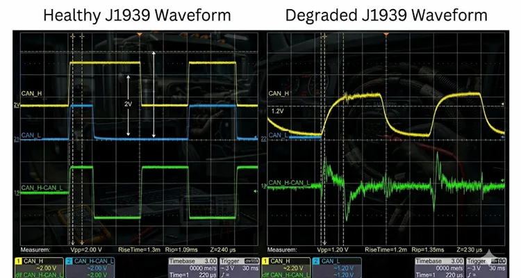
- If in doubt, scope it. A healthy J1939 waveform shows clean, square transitions with a differential voltage of approximately 2 V during dominant bits and minimal ringing. Degraded signals show rounded edges, reduced amplitude, or excessive noise.
What “fixed” actually looks like
After a repair, verify three things before releasing the equipment:
- Resistance returns to 60 Ω ±5% (with the understanding that 62–64 Ω is acceptable on legacy systems)
- Voltage levels on CAN_H and CAN_L rest at ~2.5 V (recessive)
- All previously inactive fault codes clear and stay cleared through a full key cycle
If you’ve replaced a harness section, perform a complete continuity check on all conductors. If you’ve replaced a connector, verify proper crimping and seating — a surprising number of “new” connectors fail within weeks due to improper terminal insertion.
One final point: don’t assume a repair fixed everything. I’ve seen networks with multiple simultaneous physical layer faults — a missing termination resistor and a corroded connector, for instance. Fix one, and the network improves but still misbehaves. Always re-run the full checklist after every repair. When termination is the root cause, our guide on J1939 termination mistakes that lead to ECU replacement explains why a simple resistor check beats a four-figure module swap.
Common mistakes even good technicians make
- Measuring resistance with power still applied. You’ll get meaningless readings and potentially damage your meter.
- Assuming the 9-pin connector is the correct test point. Private CAN networks often use different pins (F & G, or H & J). Know your network topology before probing.
- Replacing ECUs without verifying the physical layer. I cannot emphasize this enough. Module replacement is the most expensive and least effective way to diagnose J1939 problems.
- Overlooking aftermarket devices. Telematics units, GPS trackers, and auxiliary displays can inject noise or create termination errors. Disconnect them first when troubleshooting.
Tools that earn their keep
You don’t need a $10,000 scope. A quality automotive multimeter with min/max recording covers 80% of physical layer diagnostics. An entry-level USB oscilloscope with CAN decoding capability covers the rest. The difference between these tools and a scan-only approach is the difference between hours of diagnosis and days of guesswork.
When the physical layer is fine but the problem persists
Occasionally you’ll verify perfect resistance, clean voltages, and textbook waveforms — yet the network still misbehaves. This is when you move up the stack: check for duplicate source addresses (every ECU must have a unique address), verify all nodes are configured for the same baud rate (250 kbit/s standard for J1939), and look for message collisions or bus loading issues. Stub length and reflection can also masquerade as protocol errors; our analysis of J1939 termination stub length phantom faults details one such case that cost a fleet thousands.
But here’s the thing: in my experience, about 70% of “mysterious” J1939 problems that make it to our engineering desk turn out to be physical layer issues that someone skipped over. The remaining 30% are split between configuration errors, firmware incompatibilities, and genuine component failures. The numbers don’t lie.
A note from the factory floor: engineering reality vs. catalog specs
This is where the difference between a “cable” and an “engineered assembly” matters. IATF 16949 isn’t just a badge on our wall; it’s a constraint on our crimp height histogram. When we build a J1939 backbone for a mining truck OEM, the spec allows for a milliohm drift of less than 0.5 mΩ across the entire lifecycle.
We reject connectors with sub-5µ” gold flash not because they fail electrical test at the bench, but because we know after 4,000 hours of mine-site humidity, that flash will oxidize just enough to create the 137 Ω phantom you’ll be chasing on a Saturday night. Our facility operates under ISO 9001 and ISO 14001 management systems, and every assembly undergoes a 4-step inspection process with 100% functional testing in a climate-controlled, 5S-managed warehouse. We’ve watched harnesses fail in the field simply because the AWG selection didn’t account for voltage drop under full bus load, or because the twist pitch wasn’t held to spec across the entire length. For a deeper understanding of how cable shield and impedance specifications affect real-world performance, see our J1939 cable shield, impedance, and jacket specification guide.
If you’re specifying cables or harnesses for OEM applications, we offer full customization: logo, branding, length, color, and conductor gauge matched to your electrical and environmental requirements. Our engineering team provides direct support for integration questions and physical layer design — not because we’re selling something, but because the best way to prevent downtime is to get the physical layer right from the start.
The ROI conclusion
The 70% downtime reduction isn’t a marketing number. It’s what happens when you eliminate the diagnostic dead ends caused by skipping the physical layer. A 20-minute resistance and voltage check prevents days of chasing phantom faults. A scope waveform identifies signal degradation that scan tools can’t see. And a factory-built harness designed for your specific application prevents the problem from occurring in the first place. If you’re managing a fleet budget, our J1939 cable TCO fleet procurement guide demonstrates how upfront engineering spend reduces total cost of ownership.
The most expensive tool in your shop isn’t the one you buy. It’s the one you don’t use.
Frequently Asked Questions
Q1: What’s the correct resistance for a J1939 network, and why?
A healthy J1939 network measures approximately 60 Ω between CAN_H and CAN_L when the bus is unpowered and all modules are connected. This comes from two 120 Ω termination resistors appearing in parallel. A reading of 120 Ω indicates a missing termination; near 0 Ω indicates a short between the data lines. Readings between 62–64 Ω on legacy equipment are normal due to transceiver input impedance.
Q2: My multimeter shows 2.5 V on both CAN_H and CAN_L. Does this mean the network is healthy?
Not necessarily. A multimeter averages voltage over time and cannot display the actual waveform transitions that carry data. You could have severe signal degradation — rounded edges, excessive ringing, intermittent dropouts — and still read 2.5 V on a meter. An oscilloscope is required to verify true signal integrity.
Q3: Why do I have multiple fault codes across different ECUs when only one component seems to have failed?
This is the “many codes from one defect” pattern common to shared-bus networks like J1939. When the physical layer is compromised, multiple ECUs simultaneously lose access to network traffic. Each logs its own “lost communication” faults, making it appear as though several modules have failed independently.
Q4: Can I test J1939 with the battery still connected?
You can measure voltage with the network powered, but resistance measurements must be performed with power completely removed. Residual voltage from ECUs can damage your meter and produce inaccurate readings. Disconnect the battery for resistance tests.
Q5: What’s the difference between public and private J1939 networks when testing?
Public J1939 networks (vehicle-wide backbone) are typically accessed at pins C and D of the 9-pin diagnostic connector. Private networks (between specific ECUs, such as engine-to-transmission) often use pins F & G or H & J. Consult the vehicle wiring diagram before probing — applying voltage to the wrong pins can damage modules. For a clear visual reference, see our J1939 wiring diagram showing CAN High and CAN Low.
Q6: How do I find which ECU has a faulty termination resistor?
Systematically disconnect modules one at a time while monitoring network resistance. When the resistance jumps from 60 Ω to 120 Ω after disconnecting a particular ECU, that module likely contains one of the termination resistors. If the resistance doesn’t change, the termination is elsewhere in the harness.
Q7: Can aftermarket telematics devices cause J1939 issues?
Yes, and they frequently do. Poorly designed telematics interfaces can inject electrical noise, create ground loops, or introduce incorrect termination. The first diagnostic step for any mysterious J1939 fault should be disconnecting all aftermarket devices and retesting.
Q8: My network resistance is 47 Ω. What does this mean?
A reading significantly below 60 Ω suggests an additional, unintended resistive path between CAN_H and CAN_L — possibly a partial short, a faulty transceiver in one ECU, or more than two termination resistors installed on the bus. It could also indicate a ground-referenced transceiver fault in a legacy module (pre-ISO 11898 compliance). On some older agriculture equipment, a failing ECU doesn’t just go silent; it pulls the recessive voltage down through its protection diodes. Disconnect the suspects one by one. If pulling one module causes resistance to snap back to 60 Ω, you’ve found the culprit — even if that module’s diagnostic memory shows zero internal CAN errors.
Q9: What’s the easiest way to locate a CAN bus short?
With power removed, measure resistance between CAN_H and CAN_L while systematically disconnecting harness segments and ECUs. When the resistance suddenly increases from near-zero to 60 Ω, you’ve isolated the fault to the segment or module you just removed from the circuit.
Q10: How often should fleets perform preventive physical layer checks?
For high-utilization equipment operating in harsh environments (construction, mining, marine), quarterly checks of termination resistance and connector integrity are prudent. At minimum, perform a physical layer verification during every scheduled service interval — it takes less than 10 minutes and catches problems before they cause downtime. Fleets running Deutsch connectors should also review our Deutsch DT and HD connector series maintenance guide to prevent environmental ingress failures.
Questions about J1939 physical layer design or OEM cable specifications? Our engineering team provides direct support for integration and customization requirements.
Contact Our Engineering Team
https://obd-cable.com/contact/
WhatsApp Technical Support
https://api.whatsapp.com/send/?phone=8617307168662&text=Need+Help%3F+Chat+linda+WhatsAPP&type=phone_number&app_absent=0
