J1939 Sampling Point Diagnostics: Correlating Oscilloscope Waveform to CAN Controller Bit Timing Errors

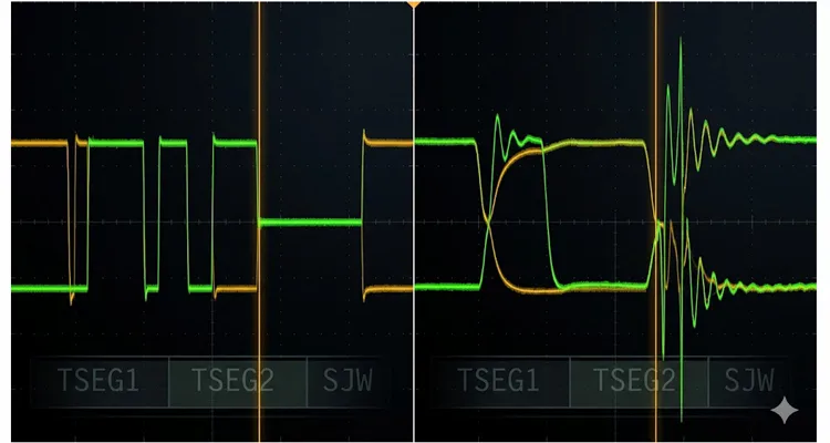
I remember the job that pushed me to sit down and write this. Third shift, a mining haul truck dead in the service bay, and the diagnostic laptop blinking J1939 No Communication every thirty seconds like clockwork. The engine would catch, run for a minute or two, then the ECM would trip on a J1939 timeout and kill everything. Restart. Same loop. A field tech had already thrown an engine ECM at it. Nothing. Swapped the instrument cluster. Still the same. Six hundred miles from the nearest dealer support, and nobody had clipped a scope onto the CAN bus yet.

Over the years I’ve watched too many sharp techs run a resistance check across the bus, see something hovering near 60 ohms, measure DC levels that look about right, and then burn two days chasing phantom fault codes because the physical layer squeaked through the standard five-minute sanity check. The bus talks. Then it doesn’t. Then it only drops out when the machine is heat-soaked, or when one particular CAN frame hits the bus, or when two specific ECUs try to arbitrate at the same instant. A network that reads electrically intact by multimeter standards can absolutely harbor a bit timing fault that only surfaces under the right conditions.

When you face intermittent communication failures that survive module swaps and wiring checks intact, you’re probably looking at a bit timing mismatch between nodes. The fastest way to prove it is by correlating oscilloscope waveform to CAN controller bit timing — lining up what the oscilloscope screen reveals with what the CAN controller believes it’s seeing during each bit.

Inside this article: How to spot a sampling point error by reading the CAN waveform raw, what the controller error counters are trying to tell you, and a step-by-step method for matching what the scope captures to what the bit timing registers actually hold. No product pitches. No theory for its own sake. Just what I’ve picked up diagnosing J1939 networks that other people walked away from.

The Scene When Sampling Point Goes Wrong

Here’s something about J1939 protocol that never found its way onto the laminated quick-reference cards. A CAN node doesn’t monitor the bus state continuously. It picks exactly one instant inside each bit — one slender decision window — and whatever voltage is present on the bus at that precise moment becomes the bit value for that bit. Miss that instant by a couple hundred nanoseconds, and your node might as well be eavesdropping on a completely different conversation than the rest of the J1939 network.

The J1939 specification recommends placing this decision window between 80% and 87.5% of the bit time. That range isn’t guesswork. By the time you’ve passed 80% of a bit, any ringing kicked up by the previous edge transition ought to have died down. Sample too early and you’re catching transients instead of settled bus levels. Sample too late and there’s insufficient room left in the phase segments to absorb oscillator drift between nodes.

Here’s what a misconfigured sampling point looks like on the scope, pulled from a case I worked through on a side-tipper fleet.

The Truck That Ran Fine Cold and Threw Errors Hot

The bus was a mixed-vendor J1939 network — five nodes distributed along roughly twelve meters of CAN harness. Cold start in the yard, everything communicated flawlessly. After roughly twenty minutes of loaded operation, the transmission ECU began logging passive errors, and before long the ABS module would vanish from the bus entirely. Park the machine for ten minutes, let it cool, restart, and every fault cleared. The cycle repeated predictably enough to set your watch by.

The scope painted a perfectly normal-looking set of CAN waveforms at idle. But when we captured during the fault window, the differential signal told a different story. Edge transitions had slowed noticeably beyond what a healthy CAN transceiver should deliver. Rise times had ballooned from under one hundred nanoseconds to nearly three hundred nanoseconds. The bus was still swinging between dominant and recessive states, but the actual decision window inside each bit was being squeezed narrower and narrower as the temperature climbed.

Root cause? One node had been configured with its sampling point at 75% of the bit time. Every other node on that bus sat at 87.5% sampling point. When edge rates degraded with heat, the 75% node began sampling while the signal was still mid-flight through the transition region. It misread bits. The CAN controller fired bit errors. Error frames flooded the bus. Error counters marched upward. Eventually that node tripped into bus-off and took the whole network down with it. This is a classic case of what we describe in our deep-dive on J1939 bit sampling error reflection bus-off, where a single mismatched node can propagate errors across an otherwise healthy backbone.

The takeaway: the waveform never looked “bad” in the textbook sense. Voltages remained within spec. Differential amplitude was acceptable. But the timing of when the CAN controller sampled the bus was wrong for the actual signal shape arriving at the controller’s pins.

What You’re Looking For on the Scope

• Capture CAN_H and CAN_L on separate channels, then view the differential math channel (CAN_H minus CAN_L).
• Zoom in to a single bit period — four microseconds at 250 kbit/s, two microseconds at 500 kbit/s.
• Examine the rising and falling edges. A healthy J1939 signal on a properly terminated bus shows edges that snap cleanly, typically well under one hundred nanoseconds.
• If edges appear rounded, stretched, or display pronounced ringing that persists beyond twenty to thirty percent of the bit width, your sampling point position becomes the critical variable.

When edges drag or ringing lingers into the back half of the bit, a controller sampling at 87.5% may still decode correctly because the signal has finally settled by that point. A controller set to sample at 60% or 70% will be reading noise. And the scope, sampling at hundreds of megasamples per second, will render the full transition beautifully — which makes it dangerously tempting to declare the signal “clean enough” when it’s anything but. Understanding this is foundational to J1939 physical layer troubleshooting with a 60-ohm waveform check, where we separate real signal integrity problems from mere configuration mismatches.

The Bit Timing Engine Under the Hood

Connecting what the oscilloscope displays to what the CAN controller actually does requires understanding how the bit timing registers work inside the silicon. This part isn’t theory. When you extract a BTR dump from a controller and hold it up against the waveform, the two either agree or they don’t. If they don’t, you’ve found your fault.

Open up a bit timing register dump and you’re staring at a small set of numbers that slice every CAN bit into discrete chunks. The controller’s peripheral clock runs through a divider to produce these chunks — the datasheets label them time quanta (Tq) — and those Tq are then allocated across several functions. Some handle synchronization with the edge from the preceding bit. Some compensate for the physical time a signal spends propagating down the harness, through connectors, through transceivers and isolators. Some give the controller room to stretch or shrink its internal timing when it detects it’s drifting out of phase with the rest of the bus. The sampling point lands precisely on the boundary between the Tq allocated for phase adjustment and the Tq held back as a timing cushion. Shift that boundary by even one Tq, and you’ve relocated the decision window.

The math itself doesn’t take long to absorb: (1 + TSEG1) / (1 + TSEG1 + TSEG2) yields the sampling point as a fraction of the bit. TSEG1 bundles the propagation segment and phase segment 1 together; TSEG2 represents phase segment 2, the timing cushion. This segment structure is laid out in detail in the CAN bus Wikipedia entry, which provides a useful reference for the bit-level architecture that every J1939 network inherits from the Bosch CAN 2.0 specification.

On paper, a controller programmed with TSEG1=13 and TSEG2=2 works out to 87.5%, same as one set to TSEG1=11 and TSEG2=4. Both nodes will acknowledge each other’s frames without complaint on a three-meter bench harness. Stretch that harness to twelve meters inside a heat-soaked mining truck, and suddenly they’re sampling different voltages at different instants within the same bit. The register math says the configurations match. The oscilloscope says otherwise, and the scope wins that argument every time.

The Silicon Interpretation Trap

Here’s where practical experience diverges from the textbook explanation. Different families of CAN controller silicon — whether it’s NXP, ST, TI, or Infineon under the hood — may interpret TSEG1 and TSEG2 slightly differently, even though the underlying arithmetic is shared. One controller where the register reads TSEG1 = 13 may genuinely program thirteen Tq before the sample point. Another where the register shows TSEG1 = 12 may add one internally in hardware, achieving exactly the same result. Copy timing values across controller families without checking the datasheet interpretation, and your sampling points can shift by several percent without anyone noticing — until the harness length grows, the temperature swings, and the bus collapses intermittently in ways no one can reproduce on the bench. We’ve seen this exact scenario play out in J1939 bit sampling error phantom fault investigations where fleets chased non-existent wiring issues for months.

Why SJW Matters More Than You Think

The SJW (Synchronization Jump Width) register matters more than most engineers give it credit for. A narrow SJW — one Tq — means the controller has almost no ability to compensate quickly for phase drift between nodes. If two ECUs on the bus are running oscillators at opposite extremes of their tolerance bands, and the SJW is set too tight, the phase error accumulates bit after bit until eventually a bit gets sampled on the wrong side of the threshold. The scope will happily display a perfectly clean signal. The controller error counters will be climbing regardless. That mismatch — clean waveform, climbing counters — is frequently your strongest clue that the problem lives in timing rather than signal integrity.

Correlating Waveform to Bit Timing: The Diagnostic Process

This is the sequence I follow when a J1939 network misbehaves and I suspect a sampling point or bit timing problem. You’ll want a four-channel oscilloscope with at least one hundred megahertz of bandwidth — two hundred is better — and differential probing capability. Serial decode is convenient but not required for the timing analysis itself. Before investing in expensive gear, consider our analysis of J1939 waveform analysis with a 200-dollar USB scope ROI — you might be surprised what entry-level tools can reveal when you know what to look for.

Start With the Waveform Capture

Connect Channel 1 to CAN_H, Channel 2 to CAN_L. Use short ground leads — spring clips landed directly on the ECU ground reference pin, not a chassis bolt half a foot away. Set the vertical scaling so the differential swing fills at least half the display. Set the timebase wide enough that three to five complete CAN frames are visible. Trigger on the start-of-frame dominant pulse: a falling edge that drops below roughly two volts on the differential channel.

Set your sample rate to at least twenty times the baud rate. For 250 kbit/s J1939, that means five megasamples per second at a minimum; ten MS/s is genuinely better. At 500 kbit/s, double both figures. If the scope is sampling too coarsely, you’ll lose the edge detail that reveals whether the signal has genuinely settled by the time the sampling point arrives.

Create the Differential Math Channel

Most scopes support a math trace: Ch1 minus Ch2. That trace is your differential signal. A healthy J1939 bus idles at roughly zero volts differential — both CAN_H and CAN_L resting near 2.5V relative to ground. During dominant bits, the differential signal swings to approximately two volts. During recessive bits, it returns to near zero.

Study that differential trace. Look for ringing that persists beyond the first fifteen to twenty percent of the bit period. Rounded edges that take longer than one hundred to one hundred fifty nanoseconds to complete the transition. Voltage steps or non-monotonic edges, which hint at a connector, termination, or transceiver problem rather than a pure timing configuration issue. We cover these waveform signatures in detail in our article on J1939 scope bench edge rates ringing differential voltage, which is useful when you need to separate physical degradation from configuration faults.

Measure One Bit Width and the Edge Timing

Use the scope cursors to measure one full bit period. At 250 kbit/s, one bit should land very near 4.00 µs. If you measure 4.10 µs or 3.90 µs, somebody has the baud rate prescaler wrong. That alone can generate intermittent errors even when the sampling point percentage calculates correctly, because the bit boundaries drift steadily relative to every other node on the bus.

Now measure rise time from the ten percent to ninety percent points on a dominant-to-recessive transition, and fall time on the opposite edge. On a healthy, properly terminated J1939 segment, both should stay under one hundred nanoseconds. If you’re seeing rise times stretch past two hundred nanoseconds, suspect excess bus capacitance — too many nodes, incorrect termination resistors, or TVS protection diodes whose junction capacitance is loading down the bus more than expected. These same physical-layer metrics appear in our J1939 physical layer ROI guide using basic tools to cut downtime 70 percent, because catching them early prevents the timing faults we’re diagnosing here.

Pull the Actual Sampling Point From the Controller Configuration

Never assume the sampling point. Extract the real bit timing register values from each ECU on the bus. That might involve reading the BTR register over a debug interface, examining the firmware source if you have access, or using a CAN configuration tool that can query the controller settings directly.

For each node, record:

• System clock frequency
• BRP (Baud Rate Prescaler) value
• TSEG1 value
• TSEG2 value
• SJW value

Calculate the sampling point for every node. Across a healthy network they should all agree within roughly one to two percent. The J1939 standard specifies 80–87.5%, with 87.5% being the most common target in production ECUs. If one node sits at 75% while the rest are at 87.5%, you’ve identified a timing mismatch that will cause errors under specific conditions — longer bus lengths, elevated temperatures, or the addition of isolation circuitry.

 Correlate Scope Waveform to Controller Sampling Point

This is the step that ties the whole diagnosis together. Take a captured waveform and drop a vertical cursor at the exact sampling point position within a bit. On a 4 µs bit at 250 kbit/s, an 87.5% sampling point falls at 3.5 µs after the bit start. Examine the differential signal voltage at that precise instant.

Has the edge transition fully completed? Is the voltage unambiguously above the dominant threshold — roughly 1.5V differential — or below the recessive threshold — roughly 0.5V differential? If the signal is still transitioning, or if ringing is pushing the voltage across the threshold more than once near the sampling instant, the controller will misread that bit at least some of the time.

Now slide your cursor earlier, to where a mismatched node’s sampling point would fall — 75% or 3.0 µs into the bit. Compare the signal condition at that location. If the bus is still mid-transition at 75% but fully settled at 87.5%, you’ve just visually confirmed exactly why one node is logging errors while the rest of the network communicates without complaint.

Check the Error Counters

Every CAN controller maintains two error counters: the Transmit Error Counter (TEC) and the Receive Error Counter (REC). Read them whenever the diagnostic interface makes them available. A node logging passive errors — either counter above 127 — is suffering repeated bit errors, stuff errors, form errors, or CRC errors. If a single node shows climbing error counters while the rest remain at zero, and the physical waveform looks clean, bit timing is the prime suspect.

Also check bus-off status. A controller transitions to bus-off when its transmit error counter exceeds 255. If you observe a node cycling into bus-off and recovering repeatedly, and the bus wiring plus termination check out fine, you are almost certainly dealing with either a baud rate mismatch or a sampling point mismatch severe enough to produce consistent bit errors during transmission attempts.

Mistakes I’ve Made and Seen Made

I’ve made most of these myself, so I’ll spare you the lecture and just tell you what bit me.

The NXP-Versus-STM32 Trap

An SJA1000-style controller and an STM32 bxCAN peripheral both have a register labeled BTR. Both use TSEG1 and TSEG2 fields. But the NXP silicon adds one internally to the value you program. The STM32 doesn’t — or handles the offset differently depending on the specific peripheral version. I once lifted a verified configuration from one platform and dropped it directly onto the other, shifting the sampling point by six percent without realizing it. Perfect on the bench. Fell over in the machine. Took a scope on one screen and a register dump on the other, side by side, to catch the discrepancy. Read the datasheet for the specific CAN controller silicon you’re holding, not for the CAN protocol in general.

The Bench Harness Illusion

A three-meter bench harness with two nodes and clean lab power bears almost no resemblance to a twelve-meter vehicle backbone carrying five nodes, inline connectors, and switching power supply noise from a running engine. Propagation delay scales directly with cable length. A sampling point that works comfortably at three meters may sit right on the ragged edge at twelve. Validate your timing configuration with the full production harness length, or at minimum calculate the propagation budget to confirm the Prop_Seg allocation is adequate for the actual cable run. Our J1939 backbone design guide on 60-ohms derating explains how backbone topology decisions made early in a machine’s design directly affect the timing margins you’ll have available later.

 Ignoring the SJW Until It’s Too Late

SJW governs how aggressively the controller can resynchronize to track oscillator drift between nodes. Dial it down to the minimum — one Tq — and the controller becomes more resistant to noise-induced resynchronization, which sounds desirable. But it also severely limits how much phase error the controller can correct. On a J1939 network where some nodes rely on ceramic resonators rather than quartz crystals, oscillator tolerance can be substantial. A narrow SJW paired with loose oscillator tolerance accumulates phase errors across consecutive bits until intermittent bit errors appear with no obvious trigger. The scope waveform looks pristine. The error counters tell a completely different story.

Trusting the Scope Decoder’s Sample Point Setting

Most oscilloscopes offering CAN decode let you configure a sample point for the decoder. That setting controls where the scope software samples the reconstructed bit stream for display purposes only. If your scope decoder is set to 80% while the actual network nodes sample at 87.5%, the scope may decode frames perfectly even as the nodes themselves are drowning in errors — or vice versa. The decoder sample point in your scope has zero relationship to the physical controllers on the bus. Always align the scope decoder’s sample point setting with the actual node configuration you’re diagnosing.

Chasing Noise When the Problem Is Timing

When error frames start appearing, every instinct points toward hunting for noise sources, bad grounds, or wiring faults. Those are all legitimate things to check. But once you’ve verified termination resistance, confirmed clean power, and established that the wiring is intact, stop searching for a physical layer gremlin that isn’t there. Extract the bit timing configuration from each ECU. Nine times out of ten, intermittent J1939 errors that outlast a thorough physical layer inspection trace back to a timing mismatch between nodes. The scope waveform is your evidence. The root cause lives in the controller registers. This is the same diagnostic principle we apply in our guide to diagnosing a J1939 data link error in 20 minutes — rule out the physical layer first, then go after timing.

Confirming the Fix

After you’ve corrected a sampling point mismatch, clearing the error counters and walking away isn’t enough. Verify systematically.

Verify Register Consistency Across All Nodes

Confirm that every node on the bus now shares the same sampling point within one percent. That means checking the actual register values, not taking the configuration tool’s high-level summary at face value. I’ve encountered tools that display 87.5% while the raw register math works out to 86.4% because of how the software rounds intermediate values. Trust the registers, not the GUI.

Load Test the Network

Run the network under genuine load. Drive bus utilization to seventy or eighty percent if your test environment supports it. Many timing problems only reveal themselves under heavy load — more arbitration on the bus, more resynchronization events, less idle time available for error recovery between frames.

Validate Across Temperature

If the original fault appeared hot, do not validate the fix on a cold machine. Bring the system fully up to operating temperature and monitor error counters continuously for at least thirty minutes. A timing configuration that sits comfortably at room temperature can fall apart at elevated temperatures as oscillator frequencies drift and transceiver propagation delays stretch.

Compare Waveforms at Both Ends of the Bus

Capture post-fix waveforms at the nodes physically nearest to and farthest from the transmitting ECU. Compare the differential signal quality at both positions. If the far-end signal shows noticeably more edge degradation, your propagation segment may need further adjustment even though the sampling point percentage calculates correctly. This far-end measurement is essentially a J1939 voltage drop field test applied to signal quality rather than DC levels — same principle, different measurement.

Document Everything

Write down what you changed and why. Include the before-and-after register values, the calculated sampling point percentages, and a scope capture demonstrating the improved correlation between signal settling time and the new sampling position. Five years from now, when someone inherits this system, they should be able to understand exactly what was wrong and exactly how it was resolved — without having to guess.

When the Bus Needs More Than a Scope Adjustment

Sometimes the problem isn’t in the firmware configuration at all. I’ve worked through cases where the bit timing was technically correct on paper, but the physical harness or transceiver design had deteriorated to the point where no reasonable sampling point could operate reliably.

Signs that point toward the physical layer rather than bit timing:

• Rise and fall times exceeding two to three hundred nanoseconds even after confirming proper termination
• Differential voltage swing dropping below 1.5V during dominant bits
• CAN_H and CAN_L common-mode voltages drifting significantly away from 2.5V
• Visible damage, corrosion, or water ingress at inline connectors

These are the situations where having a dependable source for properly specified diagnostic cabling, connectors, and test harnesses separates a repair that lasts from one that rolls back into the bay next week. Some diagnostic paths require swapping in a known-good reference cable or a break-out test harness just to isolate whether the fault lives in the harness or inside the controllers. We’ve written a dedicated guide on J1939 transceiver failure still communicating that covers the cases where a node passes every electrical test but still corrupts the bus under specific timing conditions.

If you’re managing a fleet where multiple machines exhibit the same intermittent J1939 fault pattern, it’s worth examining whether the harness assembly carries a systematic issue — incorrect wire gauge, mismatched termination resistors, or connector pin crimping that produces intermittent high resistance under vibration. The financial case for getting ahead of these problems is laid out in our analysis of J1939 network termination stub length and its impact on 15,000-dollar maintenance costs, where small physical-layer details compound into major fleet expenses.

When Off-the-Shelf Isn’t Enough

For jobs where off-the-shelf diagnostic cables or generic harness adapters fall short — or where you need custom pinouts, non-standard lengths, or specific connector configurations to interface with legacy equipment — working with a supplier that understands J1939 at the engineering level saves days of downtime. OEM-specific harnesses and breakout boxes fabricated with proper 120-ohm controlled-impedance twisted pair, correct AWG sizing, and RoHS-compliant materials eliminate an entire category of physical-layer variables from your diagnostic process. When selecting connectors for these harnesses, our J1939 Deutsch DT HD connector guide and Deutsch connector series selection and maintenance budget impact articles provide the selection criteria we use when specifying connectors that won’t become the weak link in the signal chain. The SAE J1939 Standards Collection also provides the complete physical layer and data link layer specifications governing these backbone requirements — essential reading if you are designing or validating a harness from scratch.

We build diagnostic harnesses, J1939 interface cables, and custom CAN network adapters for heavy-duty, automotive, and industrial applications. We build these on the same production floor where we run harness programs for several heavy-duty OEMs. That means the crimp tooling stays on a calibration schedule, the cable stock lives its shelf life in a climate-controlled bay rather than baking in a hot warehouse corner, and every assembly passes a full continuity and signal check before it leaves. Not because a standard requires it — though our IATF 16949:2016 certification and ISO 14001:2015 environmental management system auditors do verify — but because a harness that passes bench testing and then fails inside the machine is just another variation of the same intermittent problem this entire article has been about.

If you need engineering support on a J1939 cabling project or want to discuss a custom harness specification, reach out through our Contact page or open a conversation on WhatsApp. No obligation, no pricing talk until we understand your requirements. Just direct, technical support from people who work with CAN bus hardware every day.

Questions I Get Asked on Service Calls

A Closing Note

If this article has helped you isolate a J1939 fault that had been consuming your troubleshooting hours, I’m glad. That’s the reason I wrote it.

We are a factory that produces diagnostic cables, J1939 interface harnesses, and custom CAN network adapters for engineers and fleet operators worldwide. We don’t sell direct to consumers, and we don’t publish pricing online because every project brings its own specifications. What we do offer is direct engineering support — someone who understands CAN bus timing, connector pinouts, AWG selection, and the difference between a harness that survives bench testing and one that endures ten thousand hours inside a mining truck.

If you’re working on a J1939 system and need cables, harnesses, or breakout adapters built to your exact requirements, we can help. OEM branding, custom lengths, specific connector configurations — all manufactured under IATF 16949, ISO 14001, and RoHS compliance.

Reach out on WhatsApp to discuss your project directly, or use our Contact page if you prefer email. Tell us what you’re working on. We’ll figure out the rest together.