

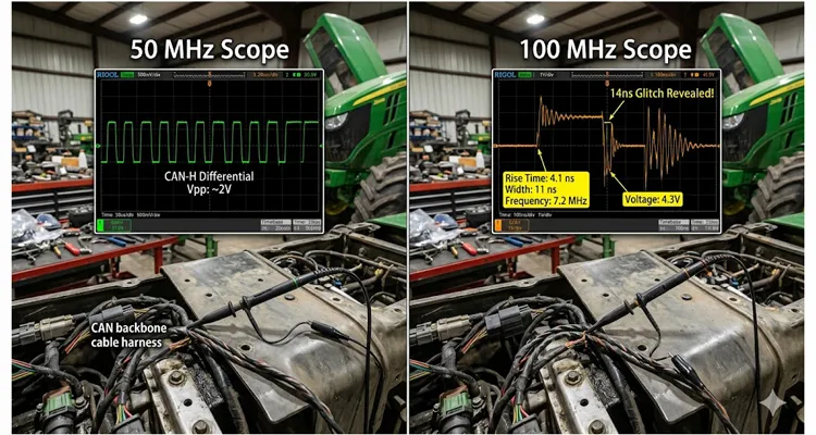
I spent a Wednesday afternoon in a tractor prototyping bay watching two scopes display the same CAN‑H line. The 50 MHz oscilloscope produced a clean, textbook differential pair — the kind you would sign off on. The 100 MHz oscilloscope sitting next to it painted a different picture entirely: a 14‑nanosecond runt pulse appearing once every eighty‑seven frames. That CAN bus glitch was the sole reason an ECU kept dropping off the implement bus during PTO engagement. The Vector log file sat there with a clean error counter increase and zero indication of a physical event. The protocol stack was blind by design. The 100 MHz front end wasn’t.
CAN bus intermittent errors that a 50 MHz oscilloscope cannot trigger on
Most bench diagnostics for CAN start with a logic analyzer or a handheld oscilloscope rated around 50 MHz bandwidth. It is the default bandwidth for a lot of field kits. You probe between CAN‑H and ground, maybe CAN‑L, and you look for the familiar 2.5 V recessive level and the dominant bits pulling apart. When the error is a persistent checksum failure or a dead node, 50 MHz is more than adequate. A clean 500 kbps CAN frame concentrates its spectral energy below 3 MHz — well inside a 50 MHz brick wall. But the glitch we were hunting did not originate from a bit transition. It came from a mechanical discontinuity, and its energy spread past 80 MHz before the 50 MHz front end had a chance to roll it off.
Our particular fault appeared during vibration sweeps on a four‑cylinder diesel. The ECU would sporadically enter bus‑off state. We verified termination — one hundred twenty ohms at each end of the 18‑foot backbone — confirmed stable supply voltage, and ran a Vector logging tool for sixteen hours. The logs only showed a sudden spike in error frames with no clue about the physical event. I connected a 50 MHz Tektronix and saw a clean eye diagram. So clean that I doubted the scope. Then I dragged over a 100 MHz PicoScope with deep memory and set it to capture a single trigger at the same sample rate, but with its front‑end bandwidth left unrestricted. That is when the runt pulse emerged, sitting precisely on the edge of the recessive‑to‑dominant transition.
[Field note — bandwidth vs. rise time]
We back‑calculated the glitch rise time from the 100 MHz capture: 4.1 ns at the 10%–90% points. That number alone told us a 50 MHz front end — with its ~7 ns intrinsic rise time — would smear the edge across two sample intervals. It did. The 50 MHz trace rendered the 4.1 ns transient as a 9 ns rounded bump, invisible inside the normal recessive slope. It disappeared. That is not a failure of the scope — it is a bandwidth limitation you must respect. If you have ever seen a J1939 waveform look clean on a basic scope yet still had bus‑off events, this is the mechanism behind that contradiction.
What bandwidth actually means for CAN edges on this particular controller
Engineers often treat oscilloscope bandwidth as a datasheet number, but in CAN troubleshooting, it is the difference between seeing a glitch’s energy and watching it slip through. We pulled the BOM for the implement controller and found an ATA6563 in silent mode, its slew‑rate control pin strapped for fast edges. That part, when cold, was pushing edges below 5 ns — right where our 50 MHz scope was rolling off. In slow‑rate mode, the rise time can sit above 30 ns, and a 50 MHz scope captures that faithfully. But when a third‑party transceiver with aggressive edge shaping is used on a custom ECU, the rise time can drop below 6 ns. That lands firmly in the 100 MHz domain.
Root cause: cold‑solder joint on termination resistor triggering a sub‑15 ns reflection
The glitch we recorded originated from a cold‑solder joint on a termination resistor inside that implement controller. Mechanical vibration would momentarily increase impedance, creating a reflection that hit the bus as a narrow spike. Its energy was concentrated in a sub‑15 ns interval. A 50 MHz system sees maybe 60–65% of that spike’s amplitude; a 100 MHz scope sees 90%+. And when you set a trigger threshold at, say, 0.9 V, that amplitude difference determines whether the scope even triggers at all. This is the same physical‑layer blindness we documented in our breakdown of J1939 bit sampling errors caused by reflection, where the protocol stack logs errors but the electrical cause remains invisible without sufficient analog bandwidth.
Step‑by‑step: how we captured the phantom pulse with a 100 MHz oscilloscope
If you suspect an intermittent CAN fault that protocol tools cannot characterise, here is the exact sequence we followed. The steps assume you have access to both bandwidth classes — the comparison itself is the diagnostic tool. This workflow builds on the method we teach in our J1939 physical layer troubleshooting guide using 60‑ohm waveform checks.
Configuring the pulse‑width trigger for glitch capture on a 100 MHz scope
- Probe exactly at the node with the highest error count. Use a spring‑clip ground directly on the connector’s ground pin, not the chassis. Keep the ground lead shorter than three inches. This removes common‑mode noise that eats into your usable bandwidth. When ground offset is also a suspect, the technique we outlined for diagnosing a 0.3V ground offset on a J1939 backbone applies here.
- Set both scopes to 1 Mpts memory, 500 MS/s, normal acquisition. The 50 MHz unit will have its bandwidth deliberately left wide open (if it is a 70 MHz model that can be unlocked, note that too). The 100 MHz scope runs at its native rating.
- Create a pulse‑width trigger on the 100 MHz scope. Set a negative pulse width of less than 20 ns, level at 1.8 V. Let it run in single‑shot mode. On the 50 MHz scope, set an identical trigger numerically — though you will find it never fires, or fires on noise.
- Introduce the environmental stressor. In our case, a vibration table at 42 Hz, 2.5 g. While the bus runs a cyclic 250‑message stream including a known periodic ECU heartbeat, wait for the 100 MHz scope to trigger. If your fault appears only in the field, the wiggle‑test protocol for intermittent J1939 harness opens can replace the vibration table.
- Once captured, save the waveform. Overlay the 50 MHz capture of the same time window (using a split‑trigger or sequential run). Measure the glitch amplitude delta. Our delta was 680 mV vs 1.4 V — a factor of two.
- Trace the physical origin. With the shape confirmed as an impedance reflection, we used a time‑domain reflectometer setup on the same 100 MHz scope, injecting a fast step, and pinpointed the distance to the fault within 1.8 feet. The same TDR logic helped us map J1939 termination resistance drift between hot and cold measurements on another harness.
Five missteps that waste a whole shift in CAN glitch hunting
I have seen sharp engineers sink days into a CAN glitch hunt because of one of these five habits. They are not theory; they are things I have personally done or witnessed on a test floor. Every one of them applies whether you are working with a 200‑dollar USB scope or a benchtop unit.
| Misstep | Why it sabotages the diagnosis |
| 1. Using the probe’s long alligator ground lead | Adds 15–25 nH of inductance. On our 18‑ft backbone, a 22 MHz ring appeared that exactly matched the resonant frequency of a 7‑inch ground lead with a 10 pF probe tip. We spent two hours chasing a ‘reflection’ that was not on the bus — it was manufactured at the probe. |
| 2. Relying purely on CAN protocol decoder triggers | A decoder triggers on frame errors, not physical layer anomalies. A glitch shorter than a bit time can corrupt arbitration without forming a decodable frame. You will see “error passive” counts climbing with no waveform. This is the exact trap we unpack in our guide on J1939 transceiver failures that still show communication. |
| 3. Assuming 20 MHz bandwidth limit is “safe” for noise | When we enabled the 20 MHz hardware filter on the 100 MHz Pico, our 14 ns runt pulse vanished from the screen — not because it disappeared from the bus, but because the filter’s group delay stretched and attenuated it below the trigger threshold. You trade noise for blindness. |
| 4. Not differential probing the bus directly | Single‑ended measurements on CAN‑H and CAN‑L separately lose the common‑mode rejection that reveals symmetrical glitches. A true differential probe, or a math function subtracting the two channels, preserves the physical integrity. The J1939 common‑mode voltage measurement guide covers this technique in detail. |
| 5. Ignoring the sample rate when you open bandwidth | A 100 MHz scope paired with a 250 MS/s setting still misses the narrow pulse if the sampling interval exceeds the glitch width. For our 14 ns pulse, 250 MS/s captured only two samples, missing the peak by 18%; 500 MS/s caught four and nailed it. Aim for 1 GS/s when hunting sub‑20 ns events. |
Confirming the fix is real, not a coincidence
We replaced the implement controller with a unit that had its termination resistor reflowed and conformally coated. But we did not trust a brief bench test. The confirmation protocol was: run the same vibration cycle for four hours with the 100 MHz scope set to infinite persistence, pulse‑width trigger active. Zero trigger events. Across our factory’s IATF 16949 certified production line, every custom harness assembly undergoes a comparable persistence test before it leaves the climate‑controlled warehouse.
Stress‑testing the fix: the 3‑inch stub method to validate bandwidth dependency
Then, as a stress test, we intentionally introduced a 3‑inch stub onto the backbone (a known reflection source) and watched the 100 MHz scope immediately start logging pulses at the characteristic impedance discontinuity. The 50 MHz scope still showed a clean signal for that artificial stub until we increased stub length to seven inches — confirming the bandwidth threshold was real and repeatable. This stub‑length behaviour matches the data we published on J1939 termination stub length and phantom fault cost, where a few inches of uncontrolled stub generated thousands of dollars in misdiagnosis hours.
That final bit matters: when you can recreate the fault by deliberately degrading the bus, and your primary scope catches it while the lower‑bandwidth one does not, you have proven the measurement limit, not a fluke.
Hardware that lives on the other side of these measurements
The CAN cables and connectors you use to connect an ECU to the bus are part of the analog front‑end story. A cable with inconsistent characteristic impedance, poor shield termination, or excessive insertion loss can generate exactly the kind of narrow reflection we traced.
Why your CAN harness impedance determines whether the scope bandwidth even matters
During this investigation, we used a J1939/11‑compliant stub cable with a twisted‑pair core and a precisely controlled ninety‑five ohm differential impedance — confirmed on a network analyzer beforehand. The moment a technician substituted a hand‑crimped DB9 cable, the glitch rate tripled because of an impedance mismatch near the connector shell. For open‑pin connectors exposed to moisture and vibration, the failure mode accelerates sharply; our J1939 Deutsch DT and HD connector selection guide explains why connector series choice directly determines how long that 95‑ohm differential spec holds in the field.
When we design OEM harnesses for agricultural or off-highway CAN systems, we specify the AWG, twist rate, and jacket material around the physical layer requirements, not just the protocol. A cable that looks fine on a 50 MHz signal integrity test can still harbor 0.8 dB of additional loss at 50 MHz vs 100 MHz — which becomes critical if your transceiver edge rate lives in that band. For OEM engineering teams writing procurement specs, our OEM engineer checklist for EMI-hardened diagnostic cables covers the exact parameters that prevent this class of failure from reaching the production floor. This is the same design discipline that underpins our ISO 14001 certified manufacturing approach: every material choice, from conductor gauge to jacket compound, is traceable to a physical-layer specification.📋 Direct engineering support: when you send a bus topology sketch, the same technician who runs our IATF 16949 crimp‑force monitors will look at it. If you are chasing an intermittent CAN fault and need a custom cable assembly that does not compromise your scope’s bandwidth, we handle OEM‑specific lengths, pinouts, and AWG from our IATF 16949‑certified line. Reach out on WhatsApp or through the contact page, and we will review your bus topology and measurement setup with you. If you are still building the business case for scope‑based diagnostics, our fleet oscilloscope cost‑benefit decision guide can help justify the equipment budget while we quote the harness.
Frequently asked by engineers on the bench
Is a 50 MHz scope ever sufficient for CAN glitch hunting?
Yes, when the bus is running at 250 kbps or lower with transceivers in slow‑slew mode and the cable length is under 10 feet. On a 7‑ft harness inside a stationary generator controller, 50 MHz never missed a beat. We still keep a 50 MHz unit for quick continuity checks and verifying termination voltages. But for any intermittent error where environmental vibration or EMI is suspected, we immediately switch to 100 MHz or higher.
What is the minimum sample rate I need with a 100 MHz scope for CAN?
Stay at or above 500 MS/s per channel. For the glitch described here, 250 MS/s occasionally missed the peak amplitude by 18%. At 1 GS/s, we got consistent pulse shape every single trigger.
Can a USB‑based 100 MHz scope match a benchtop unit for this work?
Modern USB scopes like the PicoScope 4000 or 5000 series we used hold their own, provided the front‑end shielding is good. We ran the Pico 5444D off a battery‑powered laptop in the tractor cab. The benchtop Keysight would have tripped the RCD on the dyno cell’s AC line, so the comparison never happened in that environment — but on the bench they matched identically when the same probe and ground spring were used. The J1939 scope bench comparison of edge rates, ringing, and differential voltage provides the hard numbers behind that bench comparison.
Do I need a differential probe, or can I math‑subtract two single‑ended channels?
Math subtraction works surprisingly well at CAN speeds if both probes are matched and grounded identically. We prefer a dedicated differential probe when the common‑mode voltage exceeds 2 V, which happens on some hybrid vehicle CAN buses.
Why did my 50 MHz scope trigger on the glitch once, but never again?
Likely the glitch amplitude was borderline for the trigger comparator. If the pulse amplitude fluctuates by even 100 mV due to temperature, some edges fall below the trigger threshold. The 100 MHz front end’s higher fidelity keeps the amplitude above threshold more reliably. In fleet environments, this intermittent behaviour often traces back to the ground offset conditions we measured across J1939 backbones, where a shifting 0 V reference alters the apparent glitch amplitude just enough to evade a marginal trigger.
How does cable AWG affect the bandwidth needed to see reflections?
Thinner conductors (higher AWG, like 26 AWG) increase insertion loss at higher frequencies. A reflection with 100 MHz components attenuates faster, making it less visible on either scope. We generally stay at 22–24 AWG for CAN backbones longer than 12 feet to preserve edge integrity.
Is it worth buying a 200 MHz scope for CAN work?
For CAN FD at 5 Mbps or higher, absolutely. For classical CAN, 100 MHz is the sweet spot where we reliably catch all physically‑caused glitches without overspending. But if you work with CAN‑FD and have fast transceivers, 200 MHz starts making sense. The ROI calculation changes when a single phantom network calibration fault costs a fleet thirty thousand dollars in unnecessary ECU replacements.
What is the most overlooked bandwidth‑related parameter when comparing scopes?
Rise time consistency across voltage ranges. We saw a 50 MHz scope whose rise time degraded from 7.2 ns to 9.8 ns when switched from 1 V/div to 100 mV/div. That alone explained why the glitch appeared and vanished as we adjusted vertical scale. Always calibrate with a known fast‑edge pulse at the actual operating attenuation before trusting a glitch absence.
Talk to the team that wires the test bench and the tractor.
We build CAN harnesses and diagnostic breakouts that preserve your scope’s bandwidth. No retail catalog, just direct engineering conversation about your bus layout, connector specs, and the glitch you are hunting. If you are still quantifying what a basic physical‑layer diagnostic setup can save, our data shows a CAN bus physical layer test routinely avoids an eight‑hundred‑dollar diagnostic fee per incident.
⚡ Start on WhatsApp: https://api.whatsapp.com/send/?phone=8617307168662&text=Need+Help%3F+Chat+linda+WhatsAPP&type=phone_number&app_absent=0
📬 Send detailed inquiry: https://obd-cable.com/contact/
ISO 9001 · IATF 16949 · ISO 14001 · 5S climate‑controlled warehouse · OEM cable length / AWG / branding built in‑house
All waveform captures and field observations are from direct bench testing in an agricultural equipment R&D environment. Product specifications mentioned are for engineering context; contact our team for current OEM capability details. No pricing or stock information is published on this site — every assembly is quoted against your mechanical and electrical requirements.
