

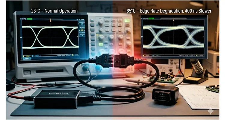
The oscilloscope screen told a story that didn’t add up.
I was standing in a test lab outside Stuttgart three years ago, staring at a CAN bus waveform on a Tektronix scope. The vehicle was a Tier 1 supplier’s next-generation telematics module—thousands of units already in field trials across Europe. The complaint was baffling: intermittent ECU communication drops, no deterministic pattern, no reproducible trigger. The fleet management team had flagged sixty-three warranty claims in six weeks. Each claim was costing roughly two hundred thirty-eight dollars to process, diagnose, and replace hardware that sometimes wasn’t broken. The running total was closing in on fifteen thousand dollars, and nobody could find the smoking gun.
What we eventually found took eight days of signal analysis, three engineers, and one moment of staring at a waveform edge that was four hundred nanoseconds too slow.
Bad components get caught. A cracked PCB, a cold solder joint, a misaligned connector—these leave forensic evidence. But when sixty-three telematics modules come back with “no trouble found” stamped on the return paperwork, you’re not hunting a manufacturing defect. You’re hunting a physics problem that your test protocols were never designed to see.
The Symptom: Sixty-Three Modules, Zero Confirmed Failures
The warranty claims had a profile that should be familiar to anyone who has worked in production-line diagnostics or fleet reliability engineering.
Vehicles would throw U-codes on the CAN bus at seemingly random intervals. Sometimes during cold starts. Sometimes after forty minutes of highway driving. Sometimes sitting idle in a parking lot with the ignition off. The telematics ECU would log a “Lost Communication with X DTC,” the module would attempt a reset, and the fault would clear. The vehicle owner would bring the car to a dealer. The dealer would run a diagnostic scan, find nothing actively wrong, and—here’s where it gets expensive—replace the telematics control unit under warranty.
Except the telematics unit wasn’t the problem. Neither was the vehicle-side harness. Neither was the connector seating. The parts coming back through reverse logistics showed no detectable failure in post-mortem analysis. They passed every functional test, every environmental stress screen, every continuity check.
This is the definition of a phantom warranty claim: a fault that appears in the field, disappears in the test lab, and generates cost without generating understanding. I’ve seen this exact pattern across multiple programs—the same ghost in the machine that drives intermittent J1939 faults right past every standard incoming inspection.
Where Standard Test Protocols Stop Looking
After ruling out the obvious—connector pin fretting, intermittent opens, thermal expansion effects on terminal contact resistance—we started looking at the one variable most production test protocols ignore: the analog shape of a digital signal.
The CAN bus in a modern vehicle operates at up to five megabits per second in CAN FD configurations. At five Mbps, a single bit period is two hundred nanoseconds. The ISO 11898-2 standard specifies that the bus driver must achieve a differential voltage swing with specific rise and fall time characteristics across a defined capacitive load. But here’s what matters in practice: if your edge rate is too slow, you don’t get a clean logic transition within the bit sampling window. The receiver sees an indeterminate voltage level at the sample point. Sometimes it resolves to a one. Sometimes it resolves to a zero. Sometimes the error handling in the CAN controller catches it and requests a retransmission. Sometimes it doesn’t, and you get a corrupted frame that passes CRC but contains garbage payload data.
The edge rate problem we eventually isolated came from an unexpected source: the OBD interface cable connecting the telematics module to the vehicle’s diagnostic bus gateway.
What We Found: The 400-Nanosecond Defect
The cable assembly in question was a custom OBD II to Molex twelve-pin diagnostic interface—a common configuration for telematics integration where the module sits behind the dashboard and connects to the vehicle bus through a pass-through harness. The assembly had passed every incoming QC check the supplier performed: 100% continuity testing, pin-to-pin mapping verification, insulation resistance measurement, and visual inspection.
What it hadn’t passed—because nobody tested for it—was a signal integrity validation under full capacitive load with the actual bus transceiver it would mate to.
The specific problem: the cable assembly was using wire with insulation that exhibited higher-than-specified dielectric constant at the operating temperature range. At room temperature on the test bench, the capacitance per meter was within spec. At sixty-five degrees Celsius—a normal temperature behind a vehicle dashboard on a summer day—the dielectric properties shifted enough to add roughly twelve picofarads per meter of additional parasitic capacitance to the bus lines.
On a three-meter cable, that doesn’t sound like much. But add it to the input capacitance of the CAN transceiver, the parasitic capacitance of the PCB traces in the telematics module, and the distributed capacitance of the vehicle-side twisted-pair bus, and suddenly you’re looking at a total capacitive load that’s pushing past the drive capability of the transceiver’s output stage.
The result: a differential signal rise time that had slowed by roughly four hundred nanoseconds. On a two-hundred-nanosecond bit period at five Mbps CAN FD, that means the signal hadn’t finished transitioning before the next bit began. The sample point—typically configured between sixty and eighty percent of the bit period in most CAN controller implementations—was landing right in the middle of the uncertain region. This is precisely the mechanism behind J1939 bit sampling errors that can push a node into bus-off without leaving a trace on a continuity tester.
This was not a cable failure in the classical sense. Continuity was perfect. Pinout was correct. Insulation resistance was well within spec. Every standard QC metric said this was a good assembly. It was, in fact, a perfectly manufactured cable that was electrically incompatible with its application environment.
Why Standard QC Misses This
Most cable assembly quality control follows a well-established protocol that hasn’t fundamentally changed in decades:
Standard QC Tests and Their Limitations
| Test | What It Verifies | What It Misses |
| 100% Continuity | No opens, no shorts, correct pin-to-pin mapping | Signal quality, impedance characteristics |
| Insulation Resistance | Dielectric integrity under DC voltage | AC dielectric behavior at operating frequency |
| Pull Force Testing | Crimp mechanical integrity | Crimp electrical performance at high frequency |
| Visual Inspection | Physical defects, label accuracy, connector seating | Everything electrical beyond DC continuity |
Each of these tests verifies DC electrical properties. None assess how the cable behaves at CAN FD operating frequencies, where bit periods are measured in hundreds of nanoseconds. These tests are necessary. For many applications, they are also sufficient. If you’re building a cable assembly for an industrial sensor that transmits a four-to-twenty-milliamp analog signal, continuity and insulation resistance are exactly what you need to verify.
But when your cable carries CAN FD at five Mbps, or LIN bus at nineteen point two kbps with tight timing tolerances, or any digital communication protocol where the bit period is measured in hundreds of nanoseconds, the DC electrical properties of the cable tell you almost nothing about how it will behave in operation.
The cable assembly that caused the phantom warranty claims I described earlier would have passed every test in the standard incoming inspection protocol of every Tier 1 supplier I’ve ever audited. That’s not an indictment of the testing—it’s a statement about the gap between what we test for and what actually causes field failures in high-speed automotive data links. The same gap exists in heavy-duty networks: a J1939 physical layer can measure a perfect sixty ohms DC termination and still produce bit errors at operating temperature because DC resistance and AC impedance are not the same measurement.
Why Edge Rates Matter More Than You Think
The physics here is straightforward, but the implications are not obvious unless you’ve spent time debugging signal integrity problems.
Every conductor in a cable assembly has distributed capacitance and inductance. The capacitance depends on the dielectric material between conductors, the geometry of the conductors, and—critically—the dielectric constant of the insulation material at the frequency and temperature of operation. Most insulation materials used in automotive wire have dielectric constants that are specified at room temperature and at low frequency (typically one kilohertz or one megahertz). But CAN FD operates with frequency components into the tens of megahertz. At those frequencies, some common insulation formulations exhibit dielectric constant shifts of five to fifteen percent. Add temperature cycling, and the shift can be even larger.
The edge rate—how fast the differential voltage transitions from recessive to dominant state and back—is a function of the transceiver’s drive strength against the total capacitive load on the bus. Slow the edge rate down by adding parasitic capacitance, and two things happen:
First, the signal eye diagram closes up. At five Mbps, a CAN FD transceiver is trying to drive a sixty-ohm differential bus with roughly thirty-five milliamps of drive current. The resulting slew rate determines the eye opening at the receiver’s sample point. Narrow the eye too much, and you get bit errors. On a benchtop scope, these degraded edges can look subtle—a slight rounding that an inexperienced tech might dismiss as probe loading rather than a systemic cable defect.
Second, and this is the subtle part that took us days to understand, the CAN controller’s error handling interacts with slow edges in ways that create the intermittent, non-deterministic failure pattern that makes phantom warranty claims so expensive to diagnose. When a bit error is detected, the CAN controller increments its transmit error counter. When that counter exceeds a threshold, the node goes into error-passive mode, limiting its ability to communicate. Eventually, if errors persist, the node goes bus-off—completely disconnected from the network. To the ECU firmware, this looks exactly like a module that has stopped communicating. The diagnostic trouble code logs point at the module, not at the cable that caused the errors.
The cable itself is perfectly functional in a DC sense. All the electrons are going where they’re supposed to go. They’re just taking four hundred nanoseconds too long to get there, and that four hundred nanoseconds is enough to push a marginal bit rate over the edge into unreliability.
A Real Failure Mode, Step by Step
Let me walk through what actually happened in the field, based on the data logs we eventually correlated with the scope measurements.
Phase One: Cold Start, Everything Works
The vehicle interior is at ambient temperature. The cable dielectric is at its nominal specified value. Total bus capacitance is within the transceiver’s drive capability. The signal eye diagram at the receiver shows clean openings with sufficient margin. Communication is error-free.
Phase Two: Warm-Up Begins
The driver has been on the road for fifteen to twenty minutes. Cabin temperature behind the dashboard starts climbing. The cable insulation’s dielectric constant begins shifting upward, adding parasitic capacitance to the bus. The edge rate starts slowing. The CAN controller’s error counters are still at zero, but the margin is eroding.
Phase Three: Threshold Crossing
Cabin temperature reaches approximately sixty-five degrees Celsius. The total bus capacitance has increased enough that the edge rate at the receiver is now borderline. The signal at the sample point occasionally falls within the indeterminate voltage range. The CAN controller detects a bit error, increments its TEC (Transmit Error Count) by eight, and requests a retransmission. The retransmission succeeds. No DTC is logged. The driver notices nothing.
Phase Four: Accumulation
Over the next thirty minutes of driving, occasional bit errors occur whenever bus traffic is heavy and the edge-rate-induced signal degradation coincides with other noise sources—a PWM-modulated LED headlight switching, an electric power steering motor drawing current, the alternator’s ripple voltage imposing noise on the vehicle’s power distribution. The TEC gradually climbs. Eventually it crosses ninety-six. The node enters error-passive mode.
Phase Five: Apparent Failure
In error-passive mode, the telematics module can only transmit passive error flags. Its ability to participate in bus arbitration is restricted. From the perspective of the other ECUs on the bus, it has gone silent. The gateway ECU logs a “Lost Communication DTC.” The vehicle owner sees a warning light and schedules a dealer visit.
Phase Six: Misdiagnosis
The dealer technician connects a diagnostic scan tool, reads the DTC, and follows the service manual procedure: replace the telematics module. The old module is returned under warranty. It goes to a failure analysis lab, where it passes every functional test at room temperature on a bench harness with different cable characteristics. The failure is attributed to “no trouble found.” The replacement module goes into the vehicle with the same marginal cable assembly. The cycle will repeat in six to eight weeks.
This six-phase cascade—from cold-start perfection to thermal failure to misdiagnosis—mirrors the pattern I documented in J1939 phantom faults caused by stub length and termination issues. The root cause differs, but the economic damage follows the same curve.
The Cable Specification Problem
The root cause here wasn’t a manufacturing defect. It was a specification gap. The OBD cable assembly had been specified with standard automotive wire that met the temperature rating and current capacity requirements but had never been characterized for high-frequency dielectric performance.
This is a common blind spot in cable assembly procurement, particularly when the assembly is being sourced as a commodity part rather than as a signal integrity-critical component. The purchasing specification called out:
- Wire gauge: twenty-two AWG
- Temperature rating: one hundred five degrees Celsius
- Connector type: OBD II male to Molex twelve-pin
- Pinout: per engineering drawing
- Continuity: one hundred percent tested
What it should have called out:
- Wire type: cross-linked polyethylene insulation, low dielectric constant grade
- Characteristic impedance: one hundred twenty ohms nominal (for CAN bus)
- Maximum intra-pair skew: less than five nanoseconds
- Maximum capacitance: specified at CAN FD operating frequency and across full temperature range
- Signal integrity validation: eye diagram measurement with representative transceiver load
The difference between those two specification approaches is the difference between procuring a cable that works on paper and procuring a cable that works in the vehicle. I’ve watched fleet operators absorb staggering maintenance costs because someone upstream treated a transmission line like a commodity extension cord.
Why Cross-Linked Polyethylene Matters
There’s a reason automotive OEMs have standardized on cross-linked polyethylene insulation for in-vehicle data bus wiring. The “cross-linking” in XLPE isn’t just a manufacturing detail—it’s a fundamental difference in dielectric behavior.
Standard thermoplastic insulation, including the PVC and TPE formulations commonly used in industrial and aftermarket cable assemblies, exhibits significant variation in dielectric constant with temperature and frequency. The polymer chains in these materials are not chemically bonded to each other. When temperature increases, the chains gain mobility, and the material’s dielectric properties shift.
Cross-linked polyethylene, by contrast, has chemical bonds between polymer chains that restrict this temperature-dependent mobility. The dielectric constant remains more stable across the automotive temperature range. The trade-off is that XLPE-insulated wire is more expensive and slightly less flexible than PVC-insulated alternatives. For a commodity OBD extension cable sold on Amazon for twelve dollars, PVC insulation is perfectly adequate. For a telematics integration harness that carries CAN FD traffic in a production vehicle, it is not.
This isn’t about “quality” in the vague sense that marketing uses the word. It’s about a specific measurable electrical characteristic that determines whether bits arrive at their destination with enough margin to survive the noise and temperature variations of real-world operation. When an aftermarket telematics installer blames the module for network errors, the real culprit is often the cable assembly degrading the physical layer.
How We Resolved It
Once we identified the root cause, the solution was straightforward in principle but required discipline in execution.
We started with a vector network analyzer connected to the assembly still installed in the vehicle—we wanted the real bus capacitance, not a benchtop estimate. The numbers confirmed what the eye diagrams had been hinting at: eighteen percent over the transceiver’s rated load at sixty-five degrees Celsius.
Wire selection came next. TXL, twenty-two AWG, SAE J1128, rated for one hundred twenty-five degrees Celsius continuous operation. The cross-linked polyethylene dropped our capacitance per meter enough to recover the margin, but we didn’t trust the datasheet alone. We built prototype assemblies and measured eye diagrams at the receiver across the full temperature range with representative bus traffic. The eye opening at sixty-five degrees Celsius improved from marginal—less than two hundred millivolts of margin at the sample point—to over six hundred millivolts. That’s the kind of margin that survives a summer heat soak in Phoenix traffic.
Then came the harder question: how do you prevent the next batch from shipping with the same invisible problem? Adding eye diagram testing to production QC isn’t trivial. It requires test equipment, fixturing, and personnel training that add cost and cycle time. We settled on a statistical sampling approach: every production lot undergoes eye diagram verification on a representative sample at elevated temperature. It’s not one hundred percent testing, but it provides statistical confidence that the manufacturing process hasn’t drifted. For assemblies carrying high-speed data, there’s no substitute. This is the same methodology behind CAN bus physical layer testing that catches marginal assemblies before they reach a vehicle.
The final step was updating the procurement specification to explicitly call out wire type, maximum capacitance, and signal integrity validation requirements. That prevents the problem from recurring even if a different supplier manufactures the assembly down the road.
The total engineering cost to find and fix this problem? Roughly forty thousand dollars in labor, equipment time, and prototype builds. The warranty claim exposure if it had gone unresolved through the full production run? An estimated two hundred fifty thousand dollars over three years. The fifteen-thousand-dollar phantom warranty claim that started the investigation was just the visible tip of a much larger iceberg.
How a Commodity Specification Reaches Production
If you’re an engineer specifying OBD cable assemblies or diagnostic harnesses for production telematics integration, certain failure patterns show up repeatedly. I’ve seen them across multiple programs and multiple suppliers.
The OBD Connector Is Standardized. The Cable Between the Connectors Is Not.
Different insulation materials, different twist geometries, and different shielding configurations produce dramatically different high-frequency behavior. Specifying only the mechanical dimensions and pinout treats the assembly like a commodity when it’s actually a transmission line. That works until the bit rate climbs past a megabit per second.
The Room-Temperature Trap
Dielectric constant specifications are almost always quoted at room temperature. Automotive applications don’t operate at room temperature. If your wire supplier can’t provide dielectric constant data at sixty-five and eighty-five degrees Celsius, the datasheet is telling you less than half the story. We’ve measured PVC-insulated assemblies that looked perfect at twenty-three degrees and fell apart at sixty-five. The same assembly, same lot, same continuity test result—completely different signal integrity at temperature.
Continuity Testing Is a DC Measurement. Signal Integrity Is a High-Frequency AC Phenomenon.
The two are almost entirely unrelated. I’ve held cables in my hands that passed continuity with flying colors and failed completely at five Mbps. Ask a continuity tester to find a four-hundred-nanosecond edge-rate defect, and it will tell you the cable is perfect. That’s not a flaw in the tester. It’s a category error in how we’ve been specifying test requirements.
The Aftermarket Cable That Works for Diagnostics but Fails in Telematics
The OBD extension cables sold for consumer use are built to a price point, not to automotive production standards. They typically use commodity PVC insulation, minimal twist control, and no signal integrity validation. For a mechanic plugging in a scan tool at room temperature for ten minutes, that’s fine. For a telematics module permanently installed behind a dashboard and communicating at five Mbps, it’s a warranty claim waiting to happen. A Deutsch 9-pin to HD Blue 26-pin cable built for Cummins ECU applications, by contrast, is engineered from the start for the thermal and vibration environment of an engine bay—exactly the standard telematics harnesses should meet.
Testing the Cable in Isolation Tells You Nothing
Until you connect it to the actual transceiver, the actual bus topology, and the actual operating environment, you haven’t validated anything that matters. System-level testing with the real hardware is non-negotiable for production applications. A J1939 backbone design works on a whiteboard; whether it works in a vehicle depends on the cable assembly connecting every node to that backbone.
How to Confirm the Fix Is Real
After you’ve identified and addressed an edge-rate-related signal integrity problem, you need to verify that the fix actually works across the full range of operating conditions. Here’s the validation protocol I’ve settled on after learning this lesson the hard way:
- Cold soak test: Soak the assembly at minus forty degrees Celsius for four hours, then run CAN FD traffic at maximum bit rate and measure eye diagram opening. The eye should be fully open with at least three hundred millivolts of margin.
- Hot soak test: Soak at eighty-five degrees Celsius for four hours, then repeat the measurement. This is where PVC-insulated cables typically fall apart. XLPE-insulated assemblies should maintain adequate eye opening.
- Thermal cycling: Cycle between minus forty and eighty-five degrees Celsius while continuously monitoring CAN error frames. The error counter should not increment during or after cycling.
- Bus loading test: Add the maximum specified number of CAN nodes to the bus and run traffic at ninety percent bus load. Verify that all nodes can communicate without error frame accumulation.
- Worst-case noise injection: This is optional but recommended for production-critical applications. Inject conducted noise per ISO 7637-2 pulse profiles and verify that the system maintains error-free communication.
If your assembly passes all five tests, you have high confidence that the fix is real and the phantom warranty claims are not coming back.
Twenty Years on a Factory Floor: What Actually Prevents This
I’ve spent two decades in cable assembly manufacturing, and if there’s one thing that separates factories that ship working product from factories that ship headaches, it’s the willingness to look past the test report and understand the application.
A continuity tester costs a few hundred dollars and tells you whether electrons can find a path from pin A to pin B. That’s necessary information, but it’s not sufficient for any application where the shape of the signal matters. Understanding signal integrity requires engineers who can read an eye diagram, who understand transmission line theory, who know why the dielectric constant of wire insulation matters at five megahertz even if it’s perfectly fine at sixty hertz. This is the difference between diagnosing a data link error in twenty minutes and chasing a ghost for three weeks.
This is why automotive production programs require IATF 16949 certification rather than just ISO 9001. The IATF standard mandates Failure Mode and Effects Analysis (FMEA) before production begins—thinking through what could go wrong rather than just inspecting for what did go wrong. A proper DFMEA for the OBD cable assembly in the telematics application would have flagged “excessive bus capacitance at operating temperature” as a potential failure mode and driven the mitigation into the specification before the first unit was ever built.
This is also why we maintain a four-step quality inspection process that goes beyond standard continuity testing: incoming material verification (including dielectric constant measurement for data-grade wire), in-process monitoring of crimp and assembly parameters, 100% electrical test, and statistical sample-based signal integrity validation for assemblies destined for high-speed data applications. Our ISO 14001 environmental management system ensures that material substitutions—which could alter dielectric properties—never happen without engineering review and requalification.
It’s not the cheapest way to build cable assemblies. It’s the way that doesn’t generate fifteen-thousand-dollar phantom warranty claims.
Questions That Come Up After You’ve Chased This Problem Once
How do I know if my OBD cable assembly has an edge rate problem?
If you’re seeing intermittent communication faults that correlate with temperature, are not reproducible on the bench at room temperature, and pass all standard continuity tests, suspect signal integrity. The definitive diagnostic is an eye diagram measurement at the receiver with the assembly at operating temperature. For J1939 networks specifically, waveform analysis with even a basic scope can reveal edge-rate degradation before it causes bus-off events.
What wire type should I specify for CAN FD OBD cable assemblies?
For production automotive applications, specify TXL or GXL wire per SAE J1128 with cross-linked polyethylene insulation. For aftermarket or diagnostic-only applications where temperature range is limited, a high-quality PVC with low dielectric constant may be adequate—but validate with measurements at your maximum operating temperature.
Can I use standard CAT5 or CAT6 cable for CAN bus?
CAT5/6 cable has a characteristic impedance of roughly one hundred ohms, which is close to CAN bus’s specified one hundred twenty ohms. The impedance mismatch is small enough that it usually works for short runs. However, CAT cable is not rated for automotive temperature or chemical exposure, and the solid conductors used in some variants are not suitable for vehicle vibration environments. Use purpose-designed automotive data bus cable for production applications.
How much does signal integrity testing add to cable assembly cost?
For production volumes, adding statistical sample-based eye diagram testing typically adds three to five percent to the unit cost. The engineering setup cost is front-loaded and amortizes across the production volume. Compare this to the cost of even one phantom warranty claim cascade, and it’s not a difficult calculation. I’ve seen basic diagnostic tools cut fleet downtime by seventy percent; the return on catching one marginal production lot before it ships is orders of magnitude higher.
Why don’t standard QC tests catch these problems?
Standard QC tests were designed for an era when cable assemblies carried analog signals or low-speed digital data. A continuity tester applies DC voltage and measures DC resistance. It has zero ability to assess how the cable behaves at five megahertz. The test equipment required for signal integrity validation—vector network analyzers, high-bandwidth oscilloscopes, calibrated test fixtures—is more expensive and requires more operator training. Most cable assembly factories don’t invest in this capability unless their customers demand it.
Is this problem specific to CAN FD, or does it affect standard CAN too?
It affects both, but CAN FD is more susceptible because of the higher bit rates—shorter bit periods mean less tolerance for slow edges. Standard CAN at five hundred kbps has bit periods of two microseconds, which provides significantly more margin for edge rate variation. However, the same dielectric-temperature mechanism applies, and a sufficiently marginal assembly can cause problems even at lower data rates. The sampling point configuration in the controller determines how much edge-rate degradation the system tolerates before errors accumulate.
What about LIN bus?
LIN operates at lower speeds, typically nineteen point two kbps, so edge rate is rarely a limiting factor. However, LIN’s single-wire physical layer means it depends on a clean ground reference. Cable assemblies with marginal ground connections can cause LIN communication faults that mimic the phantom failure pattern described here. A ground offset of even a few hundred millivolts can push single-wire transceivers outside their common-mode range.
Does cable length matter?
We measured the same PVC-insulated assembly at one meter and three meters. The shorter one passed eye diagram testing at sixty-five degrees Celsius. The longer one didn’t. The math is linear—cable capacitance is proportional to length—but the failure threshold isn’t. This is why specifying maximum capacitance rather than just wire type is important: it captures the interaction between wire properties and assembly length. The same principle governs stub length limits on J1939 backbones.
What certifications should I look for in a cable assembly supplier?
If you ask a supplier for IATF 16949 and they respond with ISO 9001, here’s the gap that matters for your signal integrity problem: ISO 9001 is a baseline quality management certification. It does not require FMEA, PPAP, or process capability analysis. IATF 16949 mandates all three, which means the supplier has been forced to think through failure modes before production rather than inspecting for them after. For this specific problem, also ask whether the supplier has in-house signal integrity validation capability and whether they can provide eye diagram measurements for your specific assembly configuration. Our facility holds full IATF 16949:2016 certification and has been ISO 14001 certified for environmental management across all production lines.
Can a continuity tester ever detect a signal integrity problem?
Ask a continuity tester to find a four-hundred-nanosecond edge-rate defect, and it will tell you the cable is perfect. That’s not a flaw in the tester. It’s a category error in how we’ve been specifying test requirements. Continuity testing measures DC resistance. Signal integrity problems are caused by AC impedance characteristics—capacitance, inductance, characteristic impedance, frequency-dependent losses. These require fundamentally different measurement techniques. A continuity tester cannot detect an edge rate problem any more than a tire pressure gauge can detect a wheel bearing failure. A transceiver that passes a loopback test but fails under bus load presents the same diagnostic blind spot.
What We Changed in Our Incoming Inspection After Stuttgart
We added one requirement to our internal process that would have caught the four-hundred-nanosecond defect before it ever reached a vehicle: every new cable assembly design destined for CAN FD or similarly high-speed automotive data links now goes through eye diagram characterization across the full operating temperature range before the first production lot ships. Not after the warranty claims start rolling in. Before.
The measurement itself isn’t complicated if you have the equipment. A vector network analyzer or a high-bandwidth scope with a differential probe, the assembly connected to the actual transceiver it will mate to, a temperature chamber cycling through the full automotive range. What you’re looking for is margin—how much eye opening remains at the worst-case temperature and bus loading condition. If the margin drops below three hundred millivolts at any point in the test, the design goes back to engineering.
Four hundred nanoseconds changed how we qualify every cable assembly that leaves this factory. If you’re specifying OBD cable assemblies for production telematics integration, or for any application where digital data moves at more than a few hundred kilobits per second, the lesson we paid fifteen thousand dollars to learn is available to you at no charge: specify the dielectric, validate the signal, and test at temperature.
Most OBD cable assemblies are specified with two numbers: pin count and length. That works until someone’s telematics fleet starts logging phantom U-codes at sixty-five degrees Celsius.
If you’d rather have the eye diagram data before the warranty claims start, we’ll run the measurements on your assembly configuration and send you the results. Same factory floor that caught the four-hundred-nanosecond defect in the first place.
Contact Page: https://obd-cable.com/contact/
OEM customization available: logo, branding, color, length, and AWG specifications. All assemblies manufactured under IATF 16949, ISO 9001, and ISO 14001 certified processes with ISO 11898-2 compliant 100% continuity testing and signal integrity validation for high-speed data applications.
