

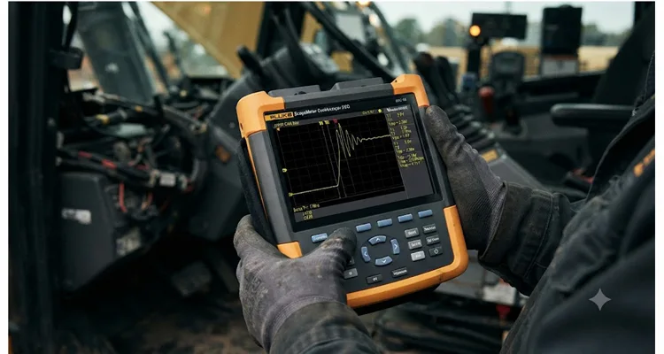
One bitter winter a few years back, I was huddled in the cab of a frozen beet harvester outside Grand Forks, watching a J1939 diagnostic screen blink “Engine Communication Lost” every 90 seconds. The error counters stayed clean between dropouts. Termination checked out. Baud rate spot on. Two ECUs had already been swapped. What eventually nailed the root cause wasn’t a fault code at all—it was a lone rising edge I snagged on a battery-powered scope running 200 MS/s, its 6-inch ground lead clipped to the nearest chassis stud. That edge carried 34% overshoot and a double-hump ring the CAN controller occasionally read as a second bit. The real culprit? A 3.5-meter unterminated stub spliced into the backbone under the cab floor, left behind after a hasty PTO retrofit.
After fifteen years spent untangling mobile machine networks, one rule has stayed constant across every ECU brand I’ve met: when J1939 frames vanish without a fault code, the problem doesn’t live in the data—it lives in the copper. Usually in one of three numbers: edge rate, overshoot, or differential voltage margin. Most people chase PGNs and address claims. The ones who solve intermittent problems for good are the ones reading the wave shape.
Your CAN Tool Said “Timeout.” The Scope Said “380 ns Rise Time.” One of Them Was Right.
Your J1939 datalogger will log a communication loss and tag it as a timeout. What it won’t tell you is that the actual culprit is a 380 ns recessive-to-dominant transition—all because a cheap spool of cable loaded so much parasitic capacitance onto the bus that the transceiver now had to fight through nearly double the intended RC time constant. It won’t show you the differential voltage sagging to 0.7 V during a ten-node burst, right as the combine’s chopper clutch engages. And it absolutely won’t reveal that 28% overshoot ringing is decaying straight across the sampling point of an NXP TJA1050 transceiver on node 3. When you trust only the protocol-level view, you end up swapping controllers that are perfectly sound while leaving the genuine physical-layer gremlins primed to strike again on the next cold morning.
Edge Rates: The Number That Predicts Bit Errors Before They Happen
I treat every J1939 transceiver as a slope-control loop, and every meter of cable as a capacitor wired in parallel with that loop. Together they set how fast the differential voltage swings from recessive to dominant. On a properly terminated 250 kbit/s J1939 backbone built to the SAE J1939-11 physical layer spec, my own field notes put a healthy rise time between 80 ns and 200 ns. Anything outside that window gets my full attention.
Rise Time vs. Cable Capacitance: The Unseen Trade-off
On our test bench, we once wound up a 40 m backbone with transceivers dialed to their fastest slew. At 500 kbit/s, the edge measured 42 ns—but the radiated emissions peak jumped 8 dB at 36 MHz, and the CAN_H to CAN_L skew widened by 4 ns simply because the cable ran past a steel enclosure. Rolling the slew back to 120 ns brought the EMI back into spec and wiped out the skew. Faster edges are only an advantage if your layout can handle the bandwidth that comes with them. Slower edges bite into the bit time and quietly strangle the receiver’s sampling window.
I once slit open a spool labeled “J1939 cable” and found a PVC jacket wrapped around completely un-twisted CAN conductors. Its capacitance measured 78 pF/m—nearly twice the 40–50 pF/m I expect from a properly twisted polyethylene dielectric. On a 40-meter backbone, that extra load dragged the rise time out to 360 ns. The bus still limped along at room temperature, but at −20°C, as the transceiver’s drive strength softened, it started coughing up sporadic CRC errors on extended frames. Every node looked guilty, and the diagnostic messages were worthless. Only the edge rate on the scope pinned the blame squarely on the cable.
My personal acceptance test for any J1939 cable assembly looks at both the rise time (10%–90% of differential swing) and the symmetry of the rising and falling edges. A properly balanced pair shows nearly identical slew rates. When the skew between CAN_H and CAN_L edges exceeds 10 ns, it points to uneven distributed capacitance or a manufacturing flaw in the twisting process—exactly the kind of defect we screen for on every production spool with a differential TDR check.
Overshoot: The Reflection You Didn’t Know You Built
Overshoot on a J1939 waveform isn’t a cosmetic bump; it’s a time-domain fingerprint of an impedance mismatch. Most often the culprit is a long stub that overstays its welcome—longer than the 1-meter guideline in the J1939-11 spec, which is an electrical limit, not a signal-purity guarantee. Once the stub length approaches a quarter wavelength of the edge’s frequency components, ringing appears, exactly as the CAN bus physical layer theory predicts for any untuned transmission line. A 3-meter unterminated stub on a 40-meter backbone? I’ve captured overshoot exceeding 40%, with three or four cycles of damped oscillation landing right where the CAN controller samples.
The Floating Backshell Problem—And What It Taught Me About Impedance Discontinuity
We once hunted a 23% overshoot that only surfaced when the backbone passed through a bulkhead connector with a zinc-plated backshell. The shell was floating—no bonding strap. It wasn’t a stub in the traditional sense, but the local impedance shift behaved identically. After bonding that shell to chassis with a 10 AWG strap, the first peak collapsed to 4%. That single repair rewired how I think about topology: any connector, splice, or bracket that introduces an impedance discontinuity can become a miniature reflection source.
One diagnostic trick I keep in the toolbox since that episode: temporarily replace the 120 Ω terminator with a split termination (two 60 Ω resistors and a capacitor to ground). It won’t cure the stub, but the change in overshoot amplitude and ring frequency reliably tells me whether I’m fighting real reflections or a transceiver oscillation. I’ve used that exact move on a sprayer bus with eight nodes to unmask a rogue stub buried inside a Y-splice mold.
Differential Voltage Thresholds: Forget the Single-Number Memes
Forget the single-number threshold memes. On a real machine carrying 18 nodes, alternator ripple, and a hydraulic manifold pulling 40 A, the voltage difference between CAN_H and CAN_L during a dominant bit will vary by 400–600 mV depending on where you probe. What matters is the worst-case noise margin you actually measure—not the theoretical receiver threshold printed in a datasheet.
Why Common-Mode Voltage Can Kill a Bus That Looks Perfect on Paper
In a heavily loaded bus with 20+ nodes, I once instrumented an 80-meter run and watched the far-end dominant differential voltage sag to 1.2 V while the source transceiver was still pumping out a healthy 2.0 V. The cable’s DC resistance and a common-mode choke were eating margin I couldn’t afford. The controllers still recognized dominant because their threshold sat at 0.9 V, but the noise margin had been shredded. Add an alternator whine or a hydraulic solenoid kickback, and that margin evaporated—producing intermittent stuff bit errors that only occurred above 1800 RPM.
Thorough waveform analysis means measuring differential voltage at multiple points under actual load. I always record the minimum dominant differential voltage, the maximum recessive differential voltage, and the common-mode voltage range. A drifting common-mode voltage—say, shifting from 2.5 V to 3.8 V because of a floating shield—can force a transceiver outside its input common-mode range even when the differential component looks clean. That exact failure mode led me to a missing shield drain connection on a Deutsch DT connector.If you’re chasing a ground offset that only appears under load, I’ve laid out a step-by-step common-mode voltage diagnosis procedure that walks you through isolating the source without shotgun ECU replacement.
A practical table I keep pinned on my toolboard, now with exactly how I measure each parameter:
| Parameter | Healthy Range (250 kbit/s) | Warning Zone | How I Measure It in the Field |
| Differential rise time (10%–90%) | 80–200 ns | 200–300 ns | Cursors on a 20 MHz bandwidth-limited differential trace, single-shot capture, leading edge of SOF |
| Overshoot (first peak) | <15% | 15–30% | Peak-to-peak with averaging off; probe at the backbone endpoint farthest from the terminator |
| Dominant differential voltage (loaded bus) | >1.5 V | 1.1–1.5 V | Measure under full electrical load—every solenoid and PWM valve active |
| Recessive differential voltage | <0.3 V | 0.3–0.5 V | Check with all nodes silent; a 0.5 V offset here often means a leaky transceiver or ground loop |
| Common-mode voltage range | 1.5–3.5 V (vs. chassis) | <1.0 or >4.0 V | Use a second channel referenced to chassis ground, DC coupled, with the engine running |
How to Capture a J1939 Waveform That Actually Tells You Something
You won’t find a multi-thousand-dollar scope on my field cart, but a short list of non-negotiable habits turns a modest instrument into a lethal diagnostic tool on J1939 networks.
Field-Proven Setup Checklist for CAN Bus Waveform Analysis
- Reach for a differential probe or two channels in math mode. Never single-ended probe CAN_H or CAN_L and assume the shape is correct. To tap into the bus cleanly without stripping insulation, I keep a J1939 breakout cable in the kit—it plugs inline and gives direct access to the signal pairs. I keep a battery-powered scope in the cab specifically to avoid ground loops; its CH1–CH2 math function gives me a clean differential trace. Keep both ground leads under 3 inches and clip them to the same chassis point as close to the measurement node as possible. With long ground leads, the common-mode rejection of the math trace collapses above 5 MHz—I’ve chased phantom ringing that vanished the instant I connected a true differential probe.
- Set your sample rate high enough to resolve rise time. For a 250 kbit/s bus, 200 MS/s is adequate for rise time and overshoot measurement, but push to 1 GS/s if you need to see the fine structure of ringing. Memory depth matters when hunting intermittent events; long record lengths capture the exact instant a solenoid fires.
- Trigger on the start-of-frame with a pulse width trigger. Set the trigger for differential >1.2 V and apply enough holdoff to isolate a clean frame. I rely on single-shot mode to grab one frame, then zoom in on the worst-case transition.
- Measure under actual load. Start the engine, engage hydraulics, toggle PTOs. A waveform that looks textbook on a quiet bench reveals nothing about the bus during a sprayer pump kick-in. I’ve recorded differential voltage sag of 300 mV exclusively at the moment six PWM valves actuated simultaneously—completely invisible in a static test.
- Save the waveform before you change anything. The trend over months is more valuable than a single snapshot. When the same machine returns six months later with a different symptom, I compare edge rates and differential levels to detect whether the cable harness is degrading.
Inside the Factory: How We Pre-Test J1939 Cables So You Don’t Chase Ghosts
On our production floor, every custom J1939 cable spool undergoes a 2-minute TDR check before the first connector is crimped. I’ve personally rejected a full spool because the impedance drifted from 118 Ω to 126 Ω over a 50 m length—a flaw a continuity tester would never flag, but which would have delivered a 19% overshoot at the far end of the backbone. We can afford to inspect every reel at that level because our IATF 16949 process control and climate-controlled 5S warehouse keep the dielectric properties stable enough that an anomaly stands out like a red flag.
From Spool to Shipment: The J1939 Cable Assembly Test Sequence
Our 4-step outgoing inspection couples that differential TDR with a swept-frequency insertion loss test and a full eye-diagram check using a real CAN transceiver load. We measure edge rate and overshoot on every spool of custom cable before cutting, and we archive the waveform records for full traceability. All our standard J1939 bulk cable features a full-plastic, RoHS-compliant jacket with a tightly controlled twist pitch—no mixed-material fillers that shift impedance with humidity. For OEM customers, we customize everything: connector brand, Deutsch or Ampseal style, length, AWG, jacket color, laser-marked branding, and even the printed legend on the outer sheath.
When a system integrator reaches us saying, “We’re seeing sporadic address claim failures on a 12-node bus,” we can cross-reference their field waveform with the production test data from their cable batch and quickly determine whether the harness is suspect or can be confidently cleared. That’s the kind of engineering partnership that transforms a J1939 cable from a commodity into a reliability-critical component.
Frequently Asked Questions From the Field
Can I use a standard oscilloscope without a differential probe?
Yes, use two channels in math mode. But here’s what most tutorials miss: with long ground leads, the common-mode rejection of the math trace breaks down above 5 MHz. I’ve seen ringing artifacts on a math trace vanish the second I connected a true differential probe. If you’re chasing overshoot above 25%, spend the extra sixty seconds to shorten the grounds to under 3 inches—otherwise you’ll tune the bus to a phantom problem.
What overshoot percentage is acceptable for a J1939 bus?
In a well-terminated backbone without long stubs, I expect less than 15%. Up to 25% is usually still functional but reveals a topology weakness that should be fixed. Above 30%, you’re gambling on temperature drift and transceiver tolerance, and the odds are not in your favor.
My recessive differential voltage sits at 0.5 V, not close to zero. Should I worry?
Yes. That offset frequently signals a partial termination failure, a leaky transceiver, or a ground potential difference between nodes. Before adding more ECUs, resolve this—every millivolt you leave on the table is noise margin you cannot afford during a high-current event.
How does cable capacitance affect J1939 rise time?
Roughly linearly: doubling the per-meter capacitance doubles the RC time constant the transceiver must drive. A 50 pF/m cable on a 50 m bus loads the driver with 2.5 nF, stretching the rise time significantly compared to a 35 pF/m cable. I always verify the capacitance spec when qualifying a new cable supplier, and if their datasheet doesn’t quote it at 1 MHz, I measure it myself.
Can I use the same waveform measurement approach for 500 kbit/s J1939?
The principles are identical, but the margins shrink. Acceptable rise times shorten, and stub tolerance drops to around 0.3 m. The faster edge makes overshoot more violent, so topology discipline becomes critical—one loose connector backshell can create more havoc at 500 kbit/s than a 2-meter stub does at 250 kbit/s.
What’s the fastest way to isolate an overshoot-causing stub?
Unplug nodes one by one while watching the differential waveform at the backbone’s endpoint. Start from the node farthest from the terminators—you’ll usually see the overshoot collapse sooner. When the overshoot suddenly drops, the last disconnected cable segment is the stub culprit. It’s a quick field method that requires no harness surgery.
Does a common-mode choke help with overshoot?
It can dampen ringing at certain frequencies, but it’s not a substitute for fixing the impedance mismatch. I’ve seen chokes successfully mask a 3-meter stub problem on the bench, only to fail once the bus expanded to 12 nodes in the field. Use a choke for EMI containment, not for topology sins.
How do I know if the J1939 transceiver itself is causing a weird waveform?
Swap the suspect node with a known-good unit or power it from an isolated supply. If the abnormal edge shape or voltage offset follows the node, the transceiver is likely damaged—I’ve identified numerous “stuck dominant” transceivers this way after nearby lightning strikes, where the waveform shows a permanently collapsed differential voltage even when the node should be silent.
What’s the difference between J1939-11 and J1939-15 physical layers from a waveform perspective?
J1939-15 runs at 100 kbit/s for longer, unshielded backbones. Edge rates are deliberately slower, so acceptable rise times relax. Overshoot tolerance is comparable, but differential voltage thresholds remain the same—do not assume you can substitute thinner wire merely because the data rate dropped. I’ve seen installers try telephone cable on a J1939-15 bus and then puzzle over why the far end sees only 0.9 V differential.
Can you build a custom J1939 harness that guarantees waveform compliance?
Absolutely. We manufacture in an IATF 16949 facility with full cable test documentation. We’ll tailor the AWG, twist pitch, shielding, connector type, and length to your bus topology, and provide pre-shipment TDR and eye-diagram reports. Just share your schematic or length requirements.
If your team is chasing intermittent J1939 issues that refuse to make sense on a diagnostic screen, or if you need a harness partner who understands signal integrity from the waveform up, send us your bus topology sketch. We’ll review it—not with a sales follow-up, but with a marked-up PDF covering impedance considerations, recommended twist pitches, and connector part numbers. Even if you don’t need a custom J1939 harness right now, you’ll walk away with a clearer picture of your physical layer.
Connect with us on WhatsApp for a direct chat about your bus layout, or use the contact form to send a drawing—we’ll get back to you with a technical review, not a pitch.
Chat on WhatsApp: https://api.whatsapp.com/send/?phone=8617307168662&text=Need+Help%3F+Chat+linda+WhatsAPP&type=phone_number&app_absent=0
Send an inquiry via Contact Page: https://obd-cable.com/contact/
